Interactive web apps with Shiny
Lecture 23
Dr. Benjamin Soltoff
Cornell University
INFO 5001 - Fall 2026
November 17, 2026
Announcements
Announcements
- Homework 06
- Project draft due Thursday
Learning objectives
- Introduce Shiny for interactive web applications
- Implement a basic Shiny app
- Introduce reactive programming concepts
- Use reactive expressions to structure an app’s logic
- Utilize {bslib} for modern Shiny UI design
- Use an AI assistant to generate Shiny code and critically evaluate it
Application exercise
ae-21
Instructions
- Go to the course GitHub org and find your
ae-21(repo name will be suffixed with your GitHub name). - Clone the repo in Positron, run
renv::restore()to install the required packages, open the Quarto document in the repo, and follow along and complete the exercises. - Render, commit, and push your edits by the AE deadline – end of the day
🔓 Decrypt the .Renviron.secret → .Renviron
source("secret.R")- The special phrase is:
info-5001
Set up Posit Assistant
Posit Assistant
- An AI assistant built into Positron that can see your R session, files, and data
- Comes with skills for specific tasks, including two for Shiny:
shiny-bslib: layouts, cards, value boxes, sidebars, navigationshiny-bslib-theming: themes, colors, fonts, dark mode
- Same idea as the skills you built last class – the assistant loads a skill only when your request matches it
⌨️ Set up Posit Assistant
Instructions
- Decrypt
.Renviron.secret(see the AE instructions), then restart R so the keys load - Copy your key: run
Sys.getenv("ANTHROPIC_API_KEY")in the console - Open the Posit Assistant pane and choose Configure AI providers (model selector, gear menu, or Command Palette)
- Select Anthropic, paste the key, and save
- Pick a Claude model and ask: “What packages are loaded in my R session?”
Posit Assistant stores the key in your system keychain, not in your project. The course OpenAI key works the same way.
05:00
Shiny: High level view
Every Shiny app has a webpage that the user visits,
and behind this webpage there is a computer that serves this webpage by running R (or Python!).

When running your app locally, the computer serving your app is your computer.

When your app is deployed, the computer serving your app is a web server.


You’ve already used Shiny
The chat apps from the LLM exercises (Clearbot demo, the quiz game) were Shiny apps built with {shinychat}.
Today we write one from scratch.
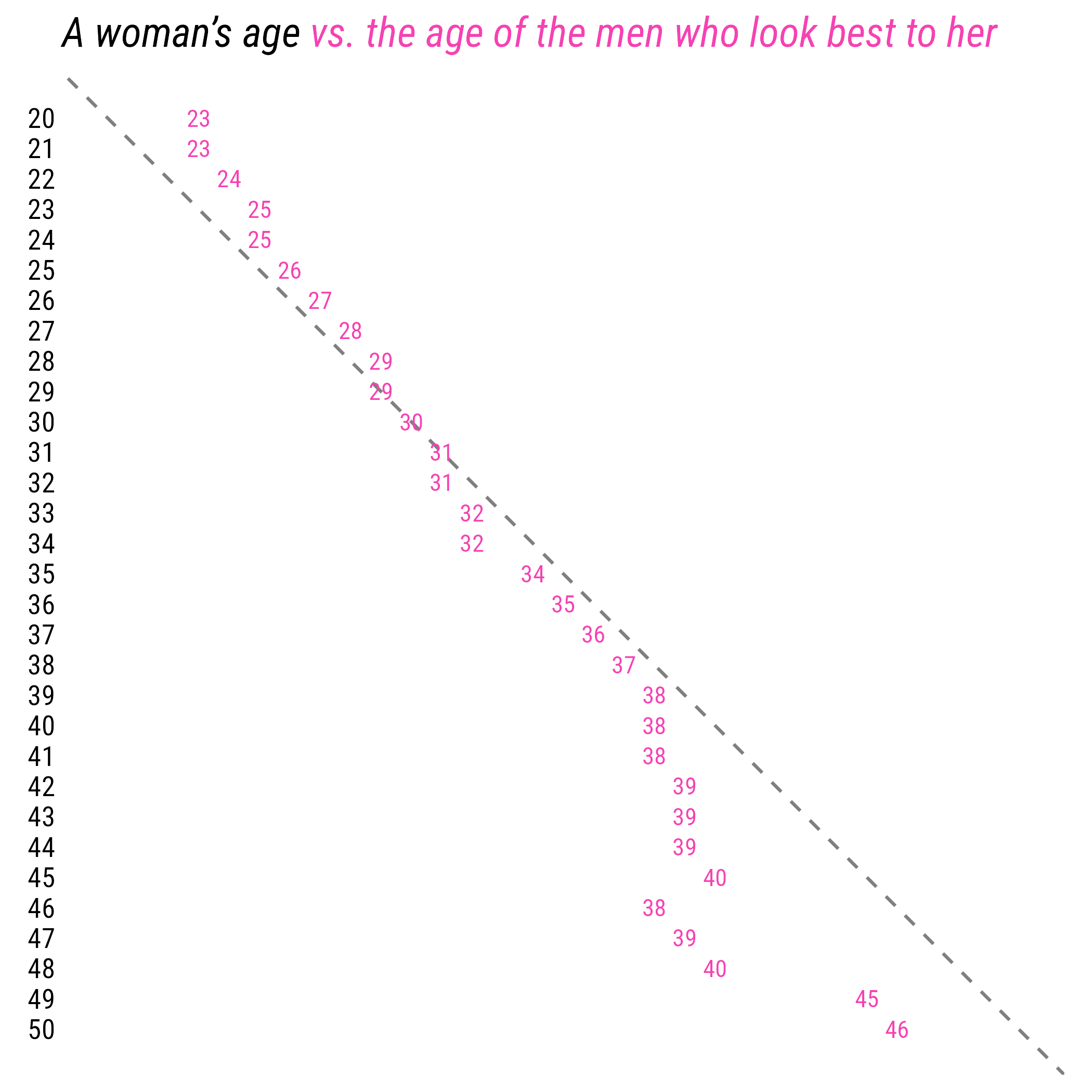
Dating rules
Age gaps
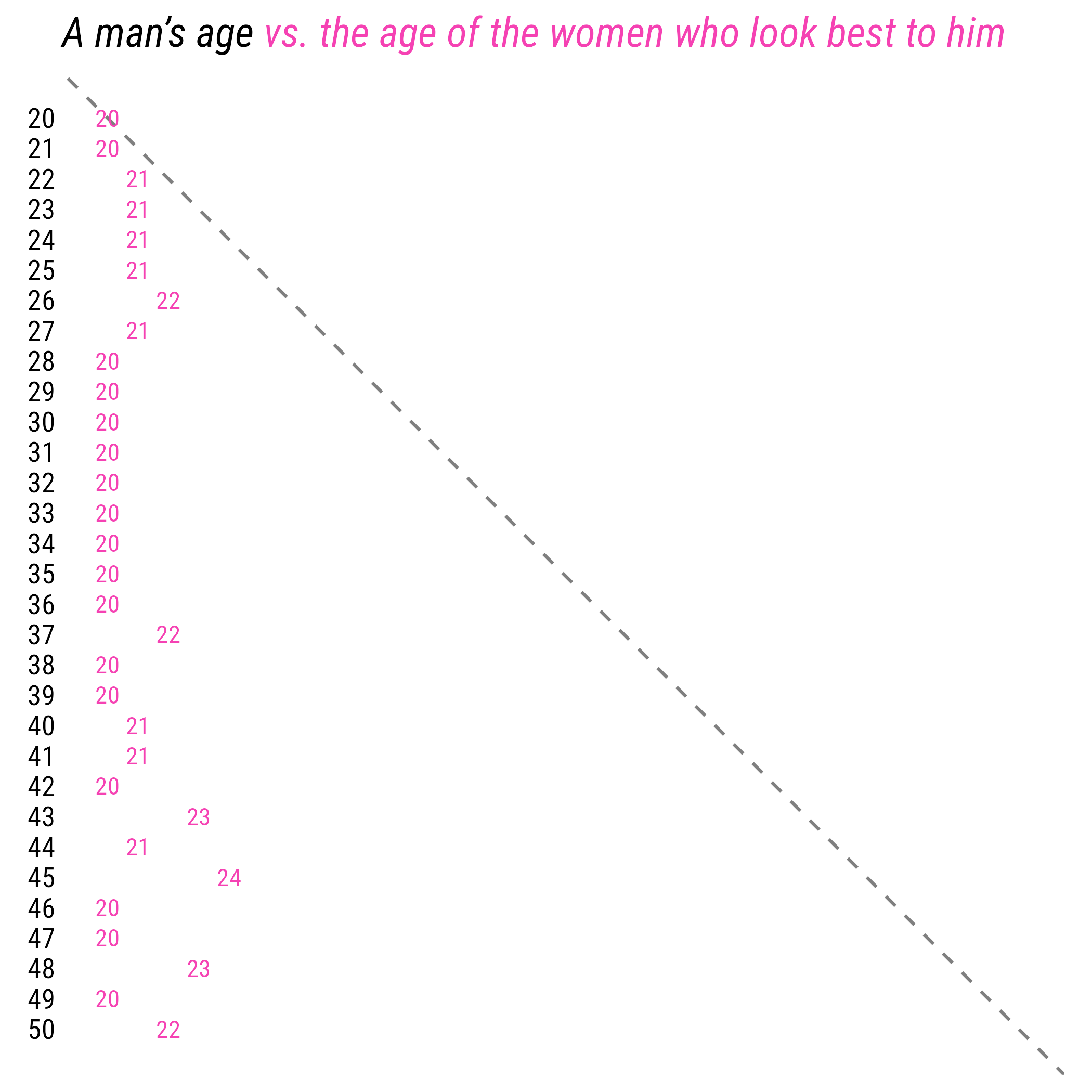
Source: Chapter 1 - Dataclysm, by Christian Rudder
Dating rules
Anatomy of a Shiny app
Shiny
- Shiny is a web application framework for R (and Python) that allows you to build interactive web applications using R (or Python) code
- Host standalone apps on a webpage, embed them in Quarto documents, or build dashboards
- Extend Shiny apps with CSS themes, {htmlwidgets}, and JavaScript actions

Learn more at https://shiny.posit.co/
{bslib}
Modern UI toolkit for Shiny based on Bootstrap
Creation of delightful and customizable Shiny dashboards with cards, value boxes, sidebars, etc.
Use of modern versions of Bootstrap and Bootswatch

Learn more at https://rstudio.github.io/bslib
Shiny + {bslib}
is now the officially recommended way to build Shiny apps.
- {shiny} functions use
camelCase - {bslib} functions use
snake_case - Older code (and many LLM answers) use
fluidPage()+sidebarLayout()from {shiny}. Both work; we use the {bslib} versions.
App components
Every Shiny app has two main components:
A UI (user interface) which controls how the app looks
and a server function which controls how the app works.
Weather data
# A tibble: 23,376 × 17
id name airport_code country state region longitude latitude date temp_avg temp_min
<dbl> <chr> <chr> <chr> <chr> <chr> <dbl> <dbl> <date> <dbl> <dbl>
1 72202 Miami KMIA US FL South -80.3 25.8 2022-01-01 24.2 21.1
2 72202 Miami KMIA US FL South -80.3 25.8 2022-01-02 24.4 21.7
3 72202 Miami KMIA US FL South -80.3 25.8 2022-01-03 22.7 17.8
4 72202 Miami KMIA US FL South -80.3 25.8 2022-01-04 20.4 16.7
5 72202 Miami KMIA US FL South -80.3 25.8 2022-01-05 22.9 19.4
6 72202 Miami KMIA US FL South -80.3 25.8 2022-01-06 21.4 16.7
7 72202 Miami KMIA US FL South -80.3 25.8 2022-01-07 23.6 20.6
# ℹ 23,369 more rows
# ℹ 6 more variables: temp_max <dbl>, precip <dbl>, snow <dbl>, wind_direction <dbl>,
# wind_speed <dbl>, air_press <dbl>Demo 01 - Our first app
💾 _demos/01_first-app.R
library(tidyverse)
library(shiny)
library(bslib)
d <- read_csv(here::here("data/weather.csv"))
ui <- page_sidebar(
title = "Temperatures at Major Airports",
sidebar = sidebar(
radioButtons(
inputId = "name",
label = "Select an airport",
choices = c(
"Hartsfield-Jackson Atlanta",
"Raleigh-Durham",
"Denver",
"Los Angeles",
"John F. Kennedy"
)
)
),
plotOutput(outputId = "plot")
)
server <- function(input, output, session) {
output$plot <- renderPlot({
d |>
filter(name %in% input$name) |>
ggplot(mapping = aes(x = date, y = temp_avg)) +
geom_line()
})
}
shinyApp(ui = ui, server = server)⌨️ Your turn - 01_first-app
Instructions
Open _exercises/01_first-app.R and run it with the Run App button. Pick a few airports to check it works.
Then modify the code:
- Add an airport that is not in
weather.csv(e.g."Ithaca"). What happens? - Replace
radioButtons()withselectInput(multiple = TRUE)orcheckboxGroupInput(). Does the plot still make sense with more than one airport? How could you fix it?
06:00
Inputs and outputs
Shiny input widgets
Shiny inputs
Shiny outputs
| Function | Outputs |
|---|---|
plotOutput() |
plot |
tableOutput() |
table |
uiOutput() |
Shiny UI element |
textOutput() |
text |
- Plots, tables, text - anything that R creates and users see
- Initialize as empty placeholder space until object is created
*Output() \(\rightarrow\) render*()
| Output function | Render function |
|---|---|
plotOutput() |
renderPlot({}) |
tableOutput() |
renderTable({}) |
uiOutput() |
renderUI({}) |
textOutput() |
renderText({}) |
The *Output() goes in the ui. The matching render*() goes in the server(), assigned to output$<id>.
Basic reactivity
Reactive elements
💾 _demos/01_first-app.R
library(tidyverse)
library(shiny)
library(bslib)

d <- read_csv(here::here("data/weather.csv"))

ui <- page_sidebar(
  title = "Temperatures at Major Airports",
  sidebar = sidebar(
    radioButtons(
      inputId = "name",
      label = "Select an airport",
      choices = c(
        "Hartsfield-Jackson Atlanta",
        "Raleigh-Durham",
        "Denver",
        "Los Angeles",
        "John F. Kennedy"
      )
    )
  ),
  plotOutput(outputId = "plot")
)

server <- function(input, output, session) {
  output$plot <- renderPlot({
    d |>
      filter(name %in% input$name) |>
      ggplot(mapping = aes(x = date, y = temp_avg)) +
      geom_line()
  })
}

shinyApp(ui = ui, server = server)Our inputs and outputs are defined by the elements in our ui.
Reactive graph
💾 _demos/01_first-app.R
library(tidyverse)
library(shiny)
library(bslib)

d <- read_csv(here::here("data/weather.csv"))

ui <- page_sidebar(
  title = "Temperatures at Major Airports",
  sidebar = sidebar(
    radioButtons(
      inputId = "name",
      label = "Select an airport",
      choices = c(
        "Hartsfield-Jackson Atlanta",
        "Raleigh-Durham",
        "Denver",
        "Los Angeles",
        "John F. Kennedy"
      )
    )
  ),
  plotOutput(outputId = "plot")
)

server <- function(input, output, session) {
  output$plot <- renderPlot({
    d |>
      filter(name %in% input$name) |>
      ggplot(mapping = aes(x = date, y = temp_avg)) +
      geom_line()
  })
}

shinyApp(ui = ui, server = server)The reactive logic is defined in our server() function - {shiny} takes care of figuring out what depends on what.
Demo 02 - adding an input
💾 _demos/02_add-input.R
library(tidyverse)
library(shiny)
library(bslib)

d <- read_csv(here::here("data/weather.csv"))

d_vars <- c(
  "Average temp" = "temp_avg",
  "Min temp" = "temp_min",
  "Max temp" = "temp_max",
  "Total precip" = "precip",
  "Snow depth" = "snow",
  "Wind direction" = "wind_direction",
  "Wind speed" = "wind_speed",
  "Air pressure" = "air_press"
)

ui <- page_sidebar(
  title = "Weather at Major Airports",
  sidebar = sidebar(
    radioButtons(
      inputId = "name",
      label = "Select an airport",
      choices = c(
        "Raleigh-Durham",
        "Houston Intercontinental",
        "Denver",
        "Los Angeles",
        "John F. Kennedy"
      )
    ),
    selectInput(
      inputId = "var",
      label = "Select a variable",
      choices = d_vars,
      selected = "temp_avg"
    )
  ),
  plotOutput(outputId = "plot")
)

server <- function(input, output, session) {
  output$plot <- renderPlot({
    d |>
      filter(name %in% input$name) |>
      ggplot(mapping = aes(x = date, y = .data[[input$var]])) +
      geom_line() +
      labs(title = str_c(input$name, " - ", input$var))
  })
}

shinyApp(ui = ui, server = server)
.data pronoun
input$var holds a column name as a string (e.g. "temp_avg"). .data[[ ]] from {rlang} lets {dplyr} and {ggplot2} use that string as a column.
More information: .data and .env pronouns
Reactive graph
With these additions, what does our reactive graph look like now?
⌨️ Your turn - 02_minmax-table
Instructions
_exercises/02_minmax-table.R is demo 02 plus the code for a table of the min and max average temperature for each year. Fill in the ____ blanks to add it to the app:
- In the
ui: the output placeholder for a table, with the idminmax - In the
server(): the matchingoutput$id andrender*()function
Run the app and switch airports. Does the table update? Does it change when you pick a new variable? Why or why not?
05:00
Reactive graph (again)
reactive()
DRY (Don’t Repeat Yourself)
Our solution repeats the filtering of d to the selected airport, once for each output.
Not a big deal here, but it adds up in larger apps: more code to keep in sync, and the same work done twice.
💾 _solutions/02_minmax-table.R
library(tidyverse)
library(shiny)
library(bslib)

d <- read_csv(here::here("data/weather.csv"))

d_vars <- c(
  "Average temp" = "temp_avg",
  "Min temp" = "temp_min",
  "Max temp" = "temp_max",
  "Total precip" = "precip",
  "Snow depth" = "snow",
  "Wind direction" = "wind_direction",
  "Wind speed" = "wind_speed",
  "Air pressure" = "air_press"
)

ui <- page_sidebar(
  title = "Weather at Major Airports",
  sidebar = sidebar(
    radioButtons(
      inputId = "name",
      label = "Select an airport",
      choices = c(
        "Raleigh-Durham",
        "Houston Intercontinental",
        "Denver",
        "Los Angeles",
        "John F. Kennedy"
      )
    ),
    selectInput(
      inputId = "var",
      label = "Select a variable",
      choices = d_vars,
      selected = "temp_avg"
    )
  ),
  plotOutput(outputId = "plot"),
  # new output placeholder
  tableOutput(outputId = "minmax")
)

server <- function(input, output, session) {
  output$plot <- renderPlot({
    d |>
      filter(name %in% input$name) |>
      ggplot(mapping = aes(x = date, y = .data[[input$var]])) +
      geom_line() +
      labs(title = str_c(input$name, " - ", input$var))
  })

  # new render function: depends on input$name only
  output$minmax <- renderTable({
    d |>
      filter(name %in% input$name) |>
      mutate(year = year(date) |> as.integer()) |>
      summarize(
        `min avg temp` = min(temp_avg),
        `max avg temp` = max(temp_avg),
        .by = year
      )
  })
}

shinyApp(ui = ui, server = server)
Demo 03 - Enter reactive()
💾 _demos/03_reactive.R
library(tidyverse)
library(shiny)
library(bslib)

d <- read_csv(here::here("data/weather.csv"))

d_vars <- c(
  "Average temp" = "temp_avg",
  "Min temp" = "temp_min",
  "Max temp" = "temp_max",
  "Total precip" = "precip",
  "Snow depth" = "snow",
  "Wind direction" = "wind_direction",
  "Wind speed" = "wind_speed",
  "Air pressure" = "air_press"
)

ui <- page_sidebar(
  title = "Weather at Major Airports",
  sidebar = sidebar(
    selectInput(
      inputId = "name",
      label = "Select airports",
      choices = sort(unique(d$name)),
      selected = "Denver",
      multiple = TRUE
    ),
    selectInput(
      inputId = "var",
      label = "Select a variable",
      choices = d_vars,
      selected = "temp_avg"
    )
  ),
  plotOutput(outputId = "plot"),
  tableOutput(outputId = "minmax")
)

server <- function(input, output, session) {
  # reactive conductor: filter once, use in both outputs
  d_city <- reactive({
    # stop quietly until at least one airport is selected
    req(input$name)

    d |>
      filter(name %in% input$name)
  })

  output$plot <- renderPlot({
    d_city() |>
      ggplot(mapping = aes(x = date, y = .data[[input$var]], color = name)) +
      geom_line() +
      labs(color = NULL)
  })

  output$minmax <- renderTable({
    d_city() |>
      mutate(year = year(date) |> as.integer()) |>
      summarize(
        `min avg temp` = min(temp_avg),
        `max avg temp` = max(temp_avg),
        .by = c(name, year)
      )
  })
}

shinyApp(ui = ui, server = server)
Reactive conductors
d_city is a reactive conductor: it sits between sources (inputs) and endpoints (outputs).
It depends on upstream inputs and returns a value that one or more downstream outputs (or other conductors) use.
Like a function in an R script, it helps you
- Avoid repeating yourself
- Break complex computations into smaller steps
- Avoid recomputing the same thing for every output
Reactive graph
reactive() tips
Written like
render*()functions, but assigned to a name instead ofoutput$
- Use its value with
react_obj(), notreact_objThink of
react_objas a function that returns the current valueForgetting the
()causes the error## Error: object of type 'closure' is not subsettable
Only usable inside reactive contexts (
render*(),reactive(),observe())## Error: Operation not allowed without an active reactive context.
Using req()
With selectInput(multiple = TRUE), the user can deselect every airport. Without protection, the app warns and draws empty output:
req() checks that a value is truthy and quietly stops the reactive if it isn’t.

Truthiness in Shiny
A value is truthy if it is:
- Not
NULL - Not
FALSE - Not an empty vector (
character(0),numeric(0), etc.) - Not an empty string
"" - Not
NA
Modern UIs with {bslib}
{bslib} components
{bslib} provides modern UI components from Bootstrap, the same library that styles Quarto HTML documents.
- Cards
- Value boxes
- Layouts (sidebars, columns, navigation)
- Popovers & tooltips
Cards
Rectangular containers with borders and padding that group related information.
Value boxes
Display a key value with a label, often a dashboard’s headline metrics.
Dynamic values in value boxes
A value box’s value can be an output, rendered on the server like any other.
Arranging components
More layouts: https://shiny.posit.co/r/layouts/
Generating Shiny apps with AI
Experimental: let the assistant write the UI
- Layout code is long, repetitive, and well documented: a good fit for an AI assistant
- The
shiny-bslibskill tells Posit Assistant to use modern {bslib} patterns instead of legacyfluidPage()code - You are still responsible for the app: does the reactive graph make sense? Does every output show what it claims?
Writing a good request
- Say what you have: “This app has a
reactive()calledd_city…” - Say what you want, concretely: “…add value boxes for average, minimum, and maximum temperature, and put the plot and table side by side in cards”
- Say what must not change: “Keep the existing inputs and the
d_cityreactive” - Ask it to run the app and fix errors
⌨️ Your turn - 03_dashboard
Instructions
_exercises/03_dashboard.R is demo 03. Ask Posit Assistant to turn it into a {bslib} dashboard with:
- value boxes for the average, minimum, and maximum temperature of the selected airports
- the plot and the min/max table in cards
Then audit the result:
- Check the numbers – select only Denver, then compute its average, minimum, and maximum temperature in the console. Do the value boxes match?
- Check the reactivity – did the new outputs reuse
d_city(), or filterdagain? - Check the edge case. – deselect every airport. Errors, warnings, or a clean empty state?
- Find one thing you would change, and change it yourself.
08:00
Discussion
- What did the assistant get right on the first try?
- Did anyone’s assistant duplicate the filtering instead of using
d_city()? - Did anyone get legacy code (
fluidPage(),renderUI()for every box)? - How did you check the app was correct, not just working?
Wrap-up
Recap
- A Shiny app is a
ui(how it looks) and aserver()(how it works) - Inputs and outputs are connected by a reactive graph that Shiny builds from your
render*()code reactive()conductors remove repetition andreq()guards against incomplete inputs- {bslib} provides modern layouts, cards, and value boxes
- An AI assistant can write the UI quickly, but you still have to check the reactive logic
Acknowledgements
- Slides derived in part from posit::conf 2025 - Shiny for R Workshop by Colin Rundel and licensed under a Creative Commons Attribution 4.0 International License.