HW 06 - Predicting attitudes towards marijuana

Homework

Modified

October 31, 2025

Important

This homework is due November 5 at 11:59pm ET.

Learning objectives

Implement resampling methods for machine learning
Estimate machine learning models for classification
Evaluate model performance using appropriate metrics
Utilize feature engineering and hyperparameter tuning to improve model performance

Getting started

Go to the info5001-fa25 organization on GitHub. Click on the repo with the prefix hw-06. It contains the starter documents you need to complete the homework.
Clone the repo and start a new workspace in Positron. See the Homework 0 instructions for details on cloning a repo and starting a new R project.

General guidance

Guidelines + tips

As we’ve discussed in lecture, your plots should include an informative title, axes should be labeled, and careful consideration should be given to aesthetic choices.

Remember that continuing to develop a sound workflow for reproducible data analysis is important as you complete the lab and other assignments in this course. There will be periodic reminders in this assignment to remind you to render, commit, and push your changes to GitHub. You should have at least 3 commits with meaningful commit messages by the end of the assignment.

Workflow + formatting

Make sure to

Update author name on your document.
Label all code chunks informatively and concisely.
Follow the Tidyverse code style guidelines.
Make at least 3 commits.
Resize figures where needed, avoid tiny or huge plots.
Turn in an organized, well formatted document.

Machine learning models are like running a marathon

They take a long time to complete. If you wait until the last minute to render your Quarto document, you will likely run out of time to submit it — especially if you wait until the slip day deadline. I highly recommend making use of code caching to store cached contents of your model code chunks so they don’t have to unnecessarily run on every render. Refer back to the slides for setting up chunk dependencies.

Data and packages

We’ll use the {tidyverse} and {tidymodels} packages for this assignment.

library(tidyverse)
library(tidymodels)

The General Social Survey is a biannual survey of the American public.

Note

The GSS gathers data on contemporary American society in order to monitor and explain trends and constants in attitudes, behaviors, and attributes. Hundreds of trends have been tracked since 1972. In addition, since the GSS adopted questions from earlier surveys, trends can be followed for up to 70 years. The GSS contains a standard core of demographic, behavioral, and attitudinal questions, plus topics of special interest. Among the topics covered are civil liberties, crime and violence, intergroup tolerance, morality, national spending priorities, psychological well-being, social mobility, and stress and traumatic events.

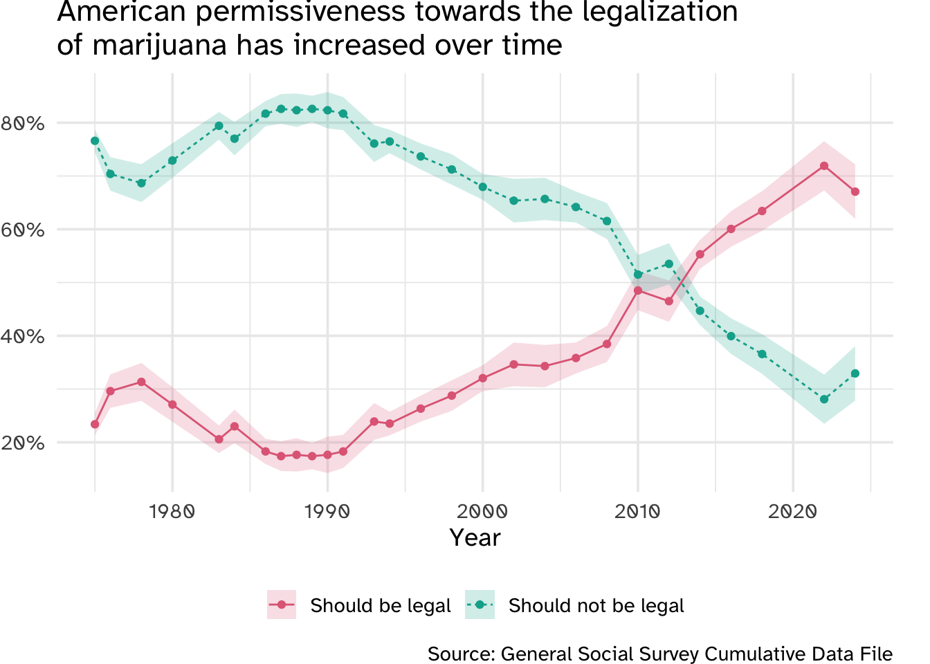
Over the past twenty years, American attitudes towards marijuana have softened extensively. In the early 2010s, the number of Americans who believed marijuana should be legal began to outnumber those who thought it should not be legal.

data/gss.rds contains a selection of variables from the 2022 and 2024 GSS.¹ The outcome of interest grass is a variable coded as either "should be legal" (respondent believes marijuana should be legal) or "should not be legal" (respondent believes marijuana should not be legal).

gss <- read_rds(file = "data/gss.rds")
skimr::skim(gss)

Data summary
Name	gss
Number of rows	1591
Number of columns	25
_______________________
Column type frequency:
factor	21
numeric	4
________________________
Group variables	None

Variable type: factor

skim_variable	n_missing	complete_rate	ordered	n_unique	top_counts
colath	836	0.47	FALSE	2	yes: 473, not: 282
colmslm	841	0.47	FALSE	2	not: 546, yes: 204
degree	0	1.00	TRUE	5	hig: 793, bac: 282, les: 207, gra: 173
fear	818	0.49	FALSE	2	no: 503, yes: 270
grass	0	1.00	FALSE	2	sho: 1105, sho: 486
gunlaw	831	0.48	FALSE	2	fav: 517, opp: 243
happy	14	0.99	TRUE	3	pre: 854, not: 389, ver: 334
health	2	1.00	FALSE	4	goo: 767, fai: 449, exc: 262, poo: 111
hispanic	15	0.99	FALSE	5	not: 1332, mex: 116, ano: 78, pue: 33
income16	179	0.89	TRUE	26	$60: 128, $50: 117, $90: 109, $17: 102
letdie1	1211	0.24	FALSE	2	yes: 265, no: 115
owngun	812	0.49	FALSE	3	no: 507, yes: 245, ref: 27
partyid	22	0.99	TRUE	8	ind: 348, str: 261, not: 219, str: 197
polviews	99	0.94	TRUE	7	mod: 537, con: 222, sli: 199, sli: 194
pray	26	0.98	FALSE	6	sev: 587, onc: 349, nev: 238, sev: 164
pres20	538	0.66	FALSE	4	bid: 598, tru: 422, oth: 28, did: 5
race	33	0.98	FALSE	3	whi: 1012, bla: 355, oth: 191
region	0	1.00	FALSE	4	sou: 663, mid: 376, wes: 302, nor: 250
sex	2	1.00	FALSE	2	fem: 861, mal: 728
sexfreq	409	0.74	TRUE	7	not: 411, 2 o: 168, 2 o: 157, onc: 144
wrkstat	3	1.00	FALSE	8	wor: 602, ret: 438, kee: 171, wor: 150

Variable type: numeric

skim_variable	n_missing	complete_rate	mean	sd	p0	p25	p50	p75	p100	hist
id	0	1.00	992.85	572.81	2	501	973	1492.5	1990	▇▇▇▇▇
age	69	0.96	52.06	18.29	18	36	53	67.0	89	▆▇▆▇▃
hrs1	844	0.47	40.10	15.65	0	35	40	47.0	89	▁▂▇▂▁
wordsum	806	0.49	5.49	2.18	0	4	6	7.0	10	▂▅▇▅▂

Tip

You can find the documentation for each of the available variables using the GSS Data Explorer. Just search by the column name to find the associated description.

Exercises

Exercise 1

Selecting potential features. For each of the variables below, explain whether or not you think they could be useful predictors for grass and why.

degree
happy
id

Now is a good time to render, commit (with a descriptive and concise commit message), and push again. Make sure that you commit and push all changed documents and your Git pane is completely empty before proceeding.

Exercise 2

Partitioning your data. Reproducibly split your data into training and test sets. Allocate 75% of observations to training, and 25% to testing. Partition the training set into 10 distinct folds for model fitting. Unless otherwise stated, you will use these sets for all the remaining exercises.

Exercise 3

Fit a null model. To establish a baseline for evaluating model performance, we want to estimate a null model. This is a model with zero predictors. In the absence of predictors, our best guess for a classification model is to predict the modal outcome for all observations (e.g. if a majority of respondents in the training set believe marijuana should be legal, then we would predict that outcome for every respondent).

The {parsnip} package includes a model specification for the null model. Fit the null model using the cross-validated folds. Report the accuracy, ROC AUC values, and confusion matrix for this model. How does the null model perform?

Exercise 4

Fit a basic logistic regression model. Estimate a simple logistic regression model to predict grass as a function of age, degree, happy, partyid, and sex. Fit the model using the cross-validated folds without any explicit feature engineering.

Report the accuracy, ROC AUC values, and confusion matrix for this model. How does this model perform?

Exercise 5

Fit a basic random forest model. Estimate a random forest model to predict grass as a function of all the other variables in the dataset (except id). In order to do this, you need to impute missing values for all the predictor columns. This means replacing missing values (NA) with plausible values given what we know about the other observations.

To do this you should build a feature engineering recipe that does the following:

Omits the id column as a predictor
Remove rows with an NA for grass - we want to omit observations with missing values for outcomes, not impute them
Use median imputation for numeric predictors
Use modal imputation for nominal predictors
Downsample the outcome of interest to have an equal number of observations for each level

Fit the model using the cross-validated folds and the ranger engine, and report the accuracy, ROC AUC values, and confusion matrix for this model. How does this model perform?

Exercise 6

Fit a nearest neighbors model. Estimate a nearest neighbors model to predict grass as a function of all the other variables in the dataset (except id). Use {recipes} to pre-process the data as necessary to train a nearest neighbors model. Be sure to also perform the same pre-processing as for the random forest model (e.g. omitting NA outcomes, imputation). Make sure your step order is correct for the recipe.

To determine the optimal number of neighbors, tune over at least 10 possible values.

Tune the model using the cross-validated folds and report the ROC AUC values for the five best models. How do these models perform?

Exercise 7

Fit a penalized logistic regression model. Estimate a penalized logistic regression model to predict grass. Use the same feature engineering recipe as for the $5$-nearest neighbors model.

Tune the model over its two hyperparameters: penalty and mixture. Create a data frame containing combinations of values for each of these parameters. penalty should be tested at the values 10^seq(-6, -1, length.out = 20), while mixture should be tested at values c(0, 0.2, 0.4, 0.6, 0.8, 1).

Tune the model using the cross-validated folds and the glmnet engine, and report the ROC AUC values for the five best models. Use autoplot() to inspect the performance of the models. How do these models perform?

Exercise 8

Tune the random forest model. Revisit the random forest model used previously. This time, implement hyperparameter tuning over the mtry and min_n to find the optimal settings. Use at least ten combinations of hyperparameter values. Report the best five combinations of values and their ROC AUC values. How do these models perform?

Exercise 9

Pick the best performing model. Select the best performing model. Train that recipe + model using the full training set and report the accuracy, ROC AUC, and confusion matrix using the held-out test set of data. Visualize the ROC curve. How would you describe this model’s performance at predicting attitudes towards the legalization of marijuana?

Bonus (optional) - Battle Royale

For those looking for a challenge (and a slight amount of extra credit for this assignment), train a high-performing model to predict grass. You must use {tidymodels} to train this model.

To evaluate your model’s effectiveness, you will generate predictions for a held-back secret test set of respondents from the survey. These can be found in data/gss-test.rds. The data frame has an identical structure to gss.rds, however I have not included the grass column. You will have no way of judging the effectiveness of your model on the test set itself.

To evaluate your model’s performance, you must create a CSV file that contains your predicted probabilities for grass. This CSV should have three columns: id (the id value for the respondent), .pred_should be legal, and .pred_should not be legal. You can generate this CSV file using the code below:

augment(best_fit, new_data = gss_secret_test) |>
  select(id, starts_with(".pred")) |>
  write_csv(file = "data/gss-preds.csv")

where gss_secret_test is a data frame imported from data/gss-test.rds and best_fit is the final model fitted using the entire training set.

Warning

Your CSV file must

Be structured exactly as I specified above.
Be stored in the data folder and named "gss-preds.csv".

If it does not meet these requirements, then you are not eligible to win this challenge.

The three students with the highest ROC AUC as calculated using their secret test set predictions will earn an extra (uncapped) 10 points on this homework assignment. For instance, if a student earned 45/50 points on the other components and was in the top-three, they would earn a 55/50 for this homework assignment.

Render, commit, and push one last time. Make sure that you commit and push all changed documents and your Git pane is completely empty before proceeding.

Wrap up

Submission

Go to http://www.gradescope.com and click Log in in the top right corner.
Click School Credentials $\rightarrow$ Cornell University NetID and log in using your NetID credentials.
Click on your INFO 5001 course.
Click on the assignment, and you’ll be prompted to submit it.
Mark all the pages associated with exercise. All the pages of your homework should be associated with at least one question (i.e., should be “checked”).
Select all pages of your .pdf submission to be associated with the “Workflow & formatting” question.

Grading

Exercise 1: 2 points
Exercise 2: 2 points
Exercise 3: 4 points
Exercise 4: 4 points
Exercise 5: 8 points
Exercise 6: 8 points
Exercise 7: 8 points
Exercise 8: 6 points
Exercise 9: 4 points
Bonus: 0 points (extra credit)
Workflow + formatting: 4 points
Total: 50 points

Workflow & formatting criteria

The “Workflow & formatting” component assesses the reproducible workflow. This includes:

Following {tidyverse} code style
All code being visible in rendered PDF without automatic wrapping (no more than 80 characters)
Appropriate figure sizing, and figures with informative labels and legends
Ensuring reproducibility by setting a random seed value.

Footnotes

For the purposes of this assignment, we will pool the observations and treat them as a single dataset.↩︎