AE 00: Visualizing the Datasaurus Dozen using the grammar of graphics and {ggplot2}
Suggested answers
These are suggested answers. This document should be used as reference only, it’s not designed to be an exhaustive key.
Packages
In this application exercise we will work with two packages:
- {datasauRus} which contains the dataset, and
- {tidyverse} which is a collection of packages for doing data analysis in a “tidy” way.
Data
The data frame we will be working with today is called datasaurus_dozen and it’s in the {datasauRus} package. Actually, this single data frame contains 13 datasets, designed to show us why data visualization is important and how summary statistics alone can be misleading. The different datasets are marked by the dataset variable.
Exercises
Exercise 1
Based on the help file, how many rows and how many columns does the datasaurus_dozen file have? What are the variables included in the data frame?
Add response here. The datasaurus_dozen dataset has 1846 rows and 3 columns. The variables include dataset (which dataset the observation comes from), x (the \(x\) value), and y (the \(y\) value).
datasaurus_dozen |>
  distinct(dataset)
# A tibble: 13 × 1
dataset
<chr>
1 dino
2 away
3 h_lines
4 v_lines
5 x_shape
6 star
7 high_lines
8 dots
9 circle
10 bullseye
11 slant_up
12 slant_down
13 wide_linesExercise 2
Plot x vs. y for the dino dataset. Then, calculate the correlation coefficient between x and y for this dataset.
Start with the datasaurus_dozen and pipe it into the filter() function to filter for observations where dataset == "dino". Store the resulting filtered data frame as a new data frame called dino_data.
dino_data <- datasaurus_dozen |>
  filter(dataset == "dino")
There is a lot going on here, so let’s slow down and unpack it a bit.
First, the pipe operator: |>, takes what comes before it and sends it as the first argument to what comes after it. So here, we’re saying filter() the datasaurus_dozen data frame for observations where dataset == "dino".
Second, the assignment operator: <-, assigns the name dino_data to the filtered data frame.
Next, we need to visualize these data. We will use the ggplot() function for this. Its first argument is the data you’re visualizing. Next we define the aesthetic mappings. In other words, the columns of the data that get mapped to certain aesthetic features of the plot, e.g. the x axis will represent the variable called x and the y axis will represent the variable called y. Then, we add another layer to this plot where we define which geometric shapes we want to use to represent each observation in the data. In this case we want these to be points, hence geom_point().
ggplot(data = dino_data, mapping = aes(x = x, y = y)) +
  geom_point() +
  labs(title = "Dino dataset")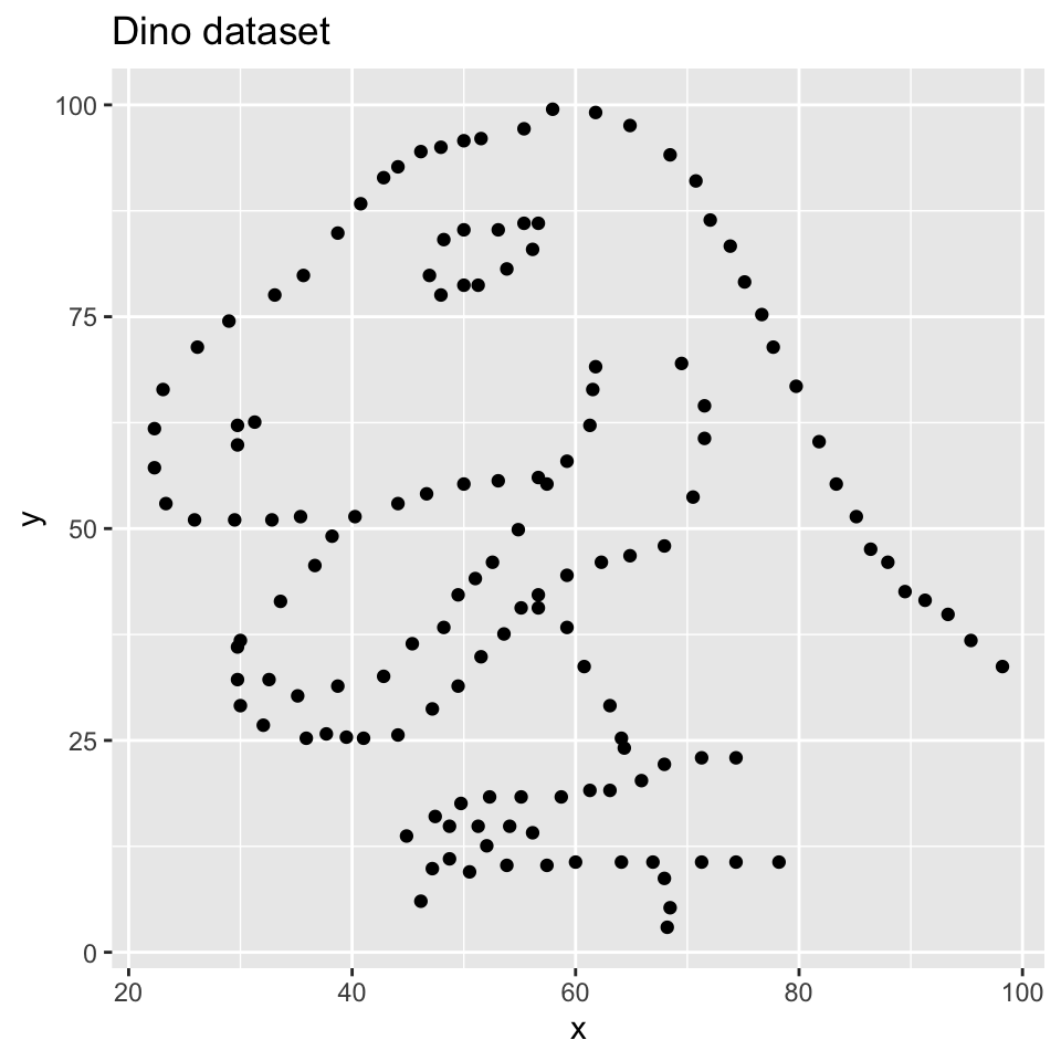
For the second part of this exercise, we need to calculate a summary statistic: the correlation coefficient. Correlation coefficient, often referred to as \(r\) in statistics, measures the linear association between two variables. You will see that some of the pairs of variables we plot do not have a linear relationship between them. This is exactly why we want to visualize first: visualize to assess the form of the relationship, and calculate \(r\) only if relevant. In this case, calculating a correlation coefficient really doesn’t make sense since the relationship between x and y is definitely not linear (it’s dinosaurial)!
For illustrative purposes only, let’s calculate the correlation coefficient between x and y.
Start with dino_data and calculate a summary statistic that we will call r as the correlation between x and y.
The correlation between \(x\) and \(y\) in the dinosaur dataset is very weak. More importantly, it is a silly measure for these variables since the relationship is clearly non-linear (i.e. T-rex-shaped).
Exercise 3
Plot x vs. y for the circle dataset. You can (and should) reuse code we introduced above, just replace the dataset name with the desired dataset. Then, calculate the correlation coefficient between x and y for this dataset. How does this value compare to the r of dino?
circle_data <- datasaurus_dozen |>
  filter(dataset == "circle")

ggplot(data = circle_data, mapping = aes(x = x, y = y)) +
  geom_point() +
  labs(title = "Circle dataset")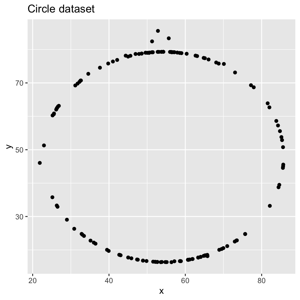
# A tibble: 1 × 1
        r
    <dbl>
1 -0.0683
Add response here. The correlation coefficient is essentially identical to that of dino, even though the shape of the data could hardly be more different.
Exercise 4
Plot x vs. y for the star dataset. You can (and should) reuse code we introduced above, just replace the dataset name with the desired dataset. Then, calculate the correlation coefficient between x and y for this dataset. How does this value compare to the r of dino?
star_data <- datasaurus_dozen |>
  filter(dataset == "star")

ggplot(data = star_data, mapping = aes(x = x, y = y)) +
  geom_point() +
  labs(title = "Star dataset")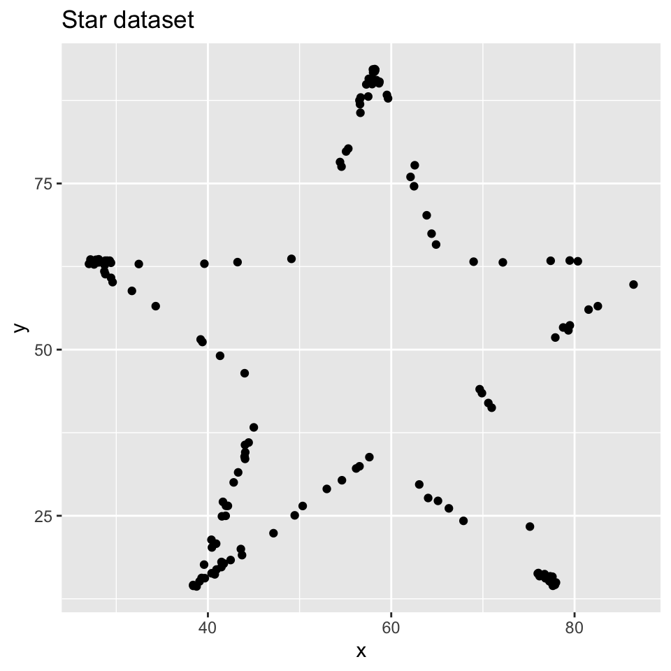
# A tibble: 1 × 1
        r
    <dbl>
1 -0.0630
Add response here. Again the correlation coefficient is nearly the same as dino and circle.
Exercise 5
Finally, plot all datasets at once.
ggplot(datasaurus_dozen, aes(x = x, y = y, color = dataset)) +
  geom_point() +
  facet_wrap(facets = vars(dataset), ncol = 3) +
  theme(legend.position = "none")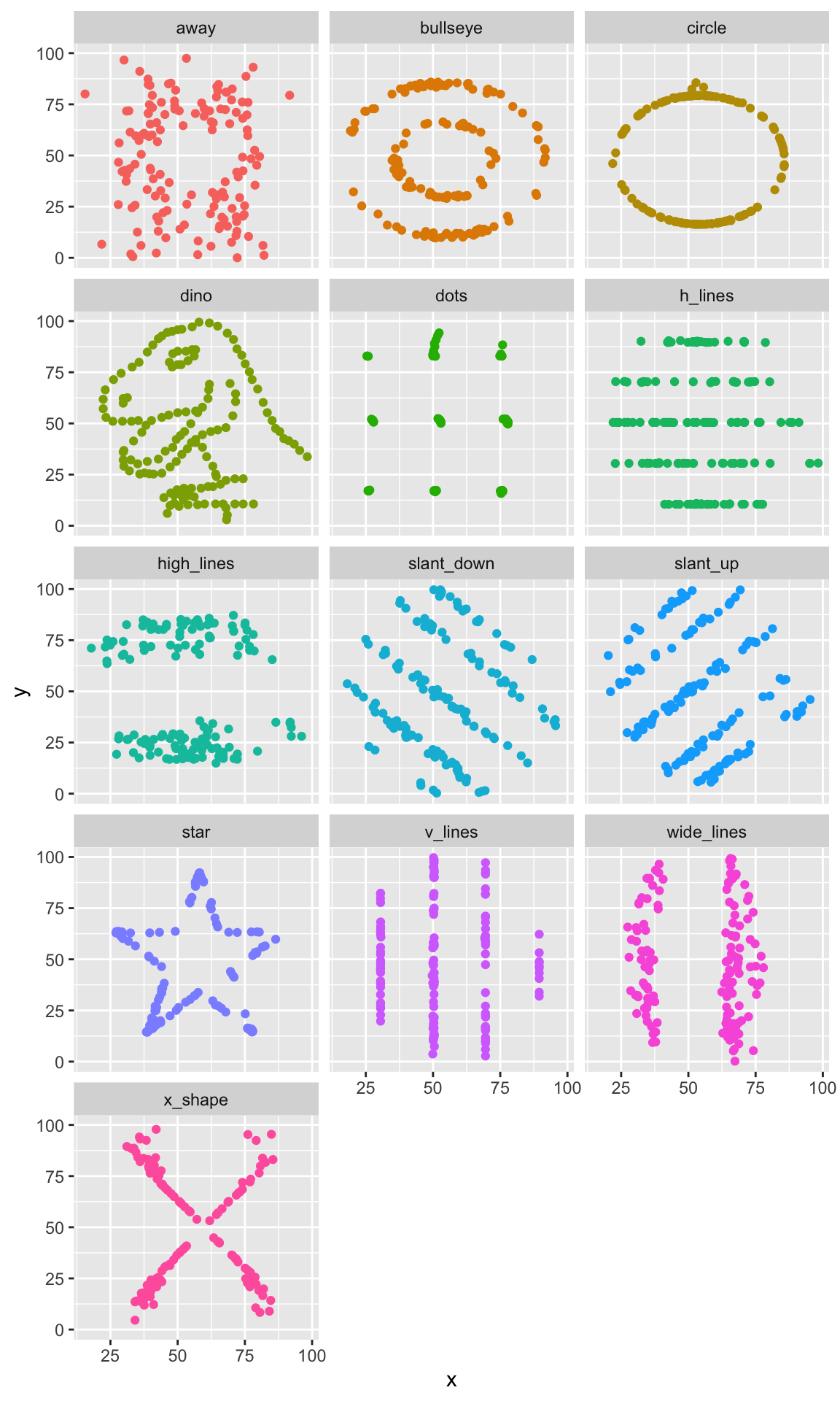
# A tibble: 13 × 2
   dataset          r
   <chr>        <dbl>
 1 away       -0.0641
 2 bullseye   -0.0686
 3 circle     -0.0683
 4 dino       -0.0645
 5 dots       -0.0603
 6 h_lines    -0.0617
 7 high_lines -0.0685
 8 slant_down -0.0690
 9 slant_up   -0.0686
10 star       -0.0630
11 v_lines    -0.0694
12 wide_lines -0.0666
13 x_shape    -0.0656
Add response here. All the datasets have a different visual pattern. However they all have approximately the same correlation coefficient. Summary statistics alone cannot tell us what a dataset looks like – we have to visualize it.
Acknowledgments
- This assignment is derived from Data Science in a Box and licensed under CC BY-SA 4.0.
sessioninfo::session_info()─ Session info ───────────────────────────────────────────────────────────────
setting value
version R version 4.6.1 (2026-06-24)
os macOS Tahoe 26.6.2
system aarch64, darwin23
ui X11
language (EN)
collate en_US.UTF-8
ctype en_US.UTF-8
tz America/New_York
date 2026-08-28
pandoc 3.10 @ /Applications/Positron.app/Contents/Resources/app/quarto/bin/tools/aarch64/ (via rmarkdown)
quarto 1.10.18 @ /Applications/quarto/bin/quarto
─ Packages ───────────────────────────────────────────────────────────────────
! package * version date (UTC) lib source
P cli 3.6.6 2026-04-09 [?] RSPM
P datasauRus * 0.1.9 2025-01-23 [?] RSPM
P digest 0.6.39 2025-11-19 [?] RSPM
P dplyr * 1.2.1 2026-04-03 [?] RSPM
P evaluate 1.0.5 2025-08-27 [?] RSPM
P farver 2.1.2 2024-05-13 [?] RSPM
P fastmap 1.2.0 2024-05-15 [?] RSPM
P forcats * 1.0.1 2025-09-25 [?] RSPM
P generics 0.1.4 2025-05-09 [?] RSPM
P ggplot2 * 4.0.3 2026-04-22 [?] RSPM
P glue 1.8.1 2026-04-17 [?] RSPM
P gtable 0.3.6 2024-10-25 [?] RSPM
P here 1.0.2 2025-09-15 [?] RSPM
P hms 1.1.4 2025-10-17 [?] RSPM
P htmltools 0.5.9 2025-12-04 [?] RSPM
P htmlwidgets 1.6.4 2023-12-06 [?] RSPM
P jsonlite 2.0.0 2025-03-27 [?] RSPM
P knitr 1.51 2025-12-20 [?] RSPM
P labeling 0.4.3 2023-08-29 [?] RSPM
P lifecycle 1.0.5 2026-01-08 [?] RSPM
P lubridate * 1.9.5 2026-02-04 [?] RSPM
P magrittr 2.0.5 2026-04-04 [?] RSPM
P otel 0.2.0 2025-08-29 [?] RSPM
P pillar 1.11.1 2025-09-17 [?] RSPM
P pkgconfig 2.0.3 2019-09-22 [?] RSPM
P purrr * 1.2.2 2026-04-10 [?] RSPM
P R6 2.6.1 2025-02-15 [?] RSPM
P RColorBrewer 1.1-3 2022-04-03 [?] RSPM
P readr * 2.2.0 2026-02-19 [?] RSPM
renv 1.2.2 2026-04-16 [1] RSPM (R 4.6.1)
P rlang 1.3.0 2026-07-05 [?] RSPM
P rmarkdown 2.31 2026-03-26 [?] RSPM
P rprojroot 2.1.1 2025-08-26 [?] RSPM
P S7 0.2.2 2026-04-22 [?] RSPM
P scales 1.4.0 2025-04-24 [?] RSPM
P sessioninfo 1.2.4 2026-06-04 [?] RSPM
P stringi 1.8.9 2026-08-04 [?] RSPM
P stringr * 1.6.0 2025-11-04 [?] RSPM
P tibble * 3.3.1 2026-01-11 [?] RSPM
P tidyr * 1.3.2 2025-12-19 [?] RSPM
P tidyselect 1.2.1 2024-03-11 [?] RSPM
P tidyverse * 2.0.0 2023-02-22 [?] RSPM
P timechange 0.4.0 2026-01-29 [?] RSPM
P tzdb 0.5.0 2025-03-15 [?] RSPM
P utf8 1.2.6 2025-06-08 [?] RSPM
P vctrs 0.7.3 2026-04-11 [?] RSPM
P withr 3.0.3 2026-06-19 [?] RSPM
P xfun 0.60 2026-07-09 [?] RSPM
P yaml 2.3.12 2025-12-10 [?] RSPM
[1] /Users/bcs88/Projects/info-5001/course-site/renv/library/macos/R-4.6/aarch64-apple-darwin23
[2] /Users/bcs88/Library/Caches/org.R-project.R/R/renv/sandbox/macos/R-4.6/aarch64-apple-darwin23/46003b10
* ── Packages attached to the search path.
P ── Loaded and on-disk path mismatch.
──────────────────────────────────────────────────────────────────────────────