HW 00 - Hello R!

Homework

Modified

August 26, 2026

Important

This homework is due September 2 at 11:59pm ET.

This homework will introduce you to the course computing workflow. The main goal is to reinforce our demo of R and Positron, which we will be using throughout the course both to learn the statistical concepts discussed in the course and to analyze real data and come to informed conclusions.

Note

R is the name of the programming language itself and Positron is a convenient interface.

An additional goal is to reinforce Git and GitHub, the collaboration and version control system that we will be using throughout the course.

Note

Git is a version control system (like “Track Changes” features from Microsoft Word but more powerful) and GitHub is the home for your Git-based projects on the internet (like DropBox but much better).

As the homeworks progress, you are encouraged to explore beyond what the homeworks dictate; a willingness to experiment will make you a much better programmer. Before we get to that stage, however, you need to build some basic fluency in R. Today we begin with the fundamental building blocks of R and Positron: the interface, reading in data, and basic commands.

Learning objectives

Familarize yourself with the workflow using R, Positron, Git, and GitHub
Write a reproducible report using Quarto
Implement version control using GitHub
Create data visualizations using {ggplot2}

Getting started

Important

Your lab TAs will lead you through the Getting Started and Packages sections.

Access Positron

If you plan to use your own computer

Make sure you have completed the software setup instructions.
Open Positron.

If you plan to use Posit Workbench

Go to https://posit-workbench.infosci.cornell.edu and log in with your Cornell NetID and Password.
Click the “New Session” button on the top of the page. Selection Positron Pro. Leave all the settings on their default state and click “Start Session”. You should now see a Positron session.

Warning

If this is your first time accessing Posit Workbench for the course, it will take a couple of minutes to prepare your session. Please be patient. When you start a session in the future, your container will already be prepared and it should start within 15 seconds.

Setup your GitHub authentication

If you are using your own computer

Run the following code in the R console to ensure you have the required packages installed:

install.packages(c("usethis", "gitcreds", "gh", "renv"))

In order to push changes to GitHub, you need to authenticate yourself. That is, you need to prove you are the owner of your GitHub account. When you log in to GitHub.com from your browser, you provide your username and password to prove your identity. But when you want to push and pull from your computer, you cannot use this method. Instead, you will prove your identity using one of two methods.

Authenticate using a Personal Access Token (PAT)

Note

This method is preferred since it allows for seamless communication between R and Git for all possible applications.

A personal access token (or PAT) is a string of characters that can be used to authenticate a user when accessing a computer system instead of a username and password. Many online services are shifting towards requiring PATs for security reasons.

With this method you will clone repositories using a regular HTTPS url like https://github.com/<OWNER>/<REPO>.git.

If you are using Posit Workbench

Configure the Git credential helper by running the following R code in the console:

usethis::use_git_config(credential.helper = "store")

Create your personal access token

Run this code from your R console:

usethis::create_github_token(
  scopes = c("repo", "user", "gist", "workflow"),
  description = "Posit Workbench",
  host = "https://github.coecis.cornell.edu/"
)

This is a helper function that takes you to the web form to create a PAT.

Give the PAT a description (e.g. “PAT for INFO 5001”)
Leave the remaining options on the pre-filled form selected and click “Generate token”. As the page says, you must store this token somewhere, because you’ll never be able to see it again, once you leave that page or close the window. For now, you can copy it to your clipboard (we will save it in the next step).

If you lose or forget your PAT, just generate a new one.

Store your PAT

In order to store your PAT so you don’t have to reenter it every time you interact with Git, we need to run the following code:

gitcreds::gitcreds_set(url = "https://github.coecis.cornell.edu/")

When prompted, paste your PAT into the console and press return. Your credential should now be saved on your computer.

Confirm your PAT is saved

Run the following code:

gh::gh_whoami(.api_url = "https://github.coecis.cornell.edu/")

usethis::git_sitrep()

You should see output that provides information about your GitHub account.

Authenticate using Secure Shell Protocol

Note

You can use this approach to authenticate yourself on GitHub. Note that you may find some limitations communicating with Git outside of standard processes (e.g. cloning/pushing/pulling repos directly), and will still need to create a PAT for some course assignments. However for students using Posit Workbench, the SSH method will work for the entire semester (i.e. set it up once and never have to worry about it again).

Instructions for authenticating with SSH

The Secure Shell Protocol (SSH) is another method for authenticating your identity when communicating with GitHub. While a password can eventually be cracked with a brute force attack, SSH keys are nearly impossible to decipher by brute force alone. Generating a key pair provides you with two long strings of characters: a public and a private key. You can place the public key on any server (like GitHub), and then unlock it by connecting to it with a client that already has the private key (your computer or Posit Workbench). When the two match up, the system unlocks without the need for a password.

The URL for SSH remotes looks like git@github.com:<OWNER>/<REPO>.git. Make sure you use this URL to clone a repository. If you accidentally use the HTTPS version, the operation will not work.

Set up your SSH key

Note

You only need to do this authentication process one time on a single system.

Type credentials::ssh_keygen() into your console.
R will ask “No SSH key found. Generate one now?” You should click 1 for yes.

You will generate a key. It will begin with “ssh-rsa….” and look something like this:

$key
[1] "/home/bcs88/.ssh/id_rsa"

$pubkey
[1] "ssh-rsa AAAAB3NzaC1yc2EAAAADAQABAAABAQDJYmJeave083exQwYcIqZJk/Y1mgPxdcTYCTWLL+6mlhN9MM3enjDqb2eZvVJ0JK29NYL1++DTqY/saP08IlswNIMntwaWFDNx42yLsuFrWiPqzm9hWWnRcor/d+4zTrcSIEvfAAnLsYkagNqurrCf2taO62YRepTgxErLvLOG10qn4LKhNfT+PTqdPq2Mr88jXQYYrRxGnOV6oVYf6PurKkiooTsKYxVtJWai8Ek9fhK2y5vaQd5yP0H/3Hbw8Mn+rB+O8Yj6/oQKGBCgxkDB4Aw7T91DkIXlHppneO683Y54WvUftJYvSVsnyt/XuNjvXNAir0+kHETLM32uzH6L"

Copy the entire string of characters (not including the quotation marks) and paste them into the settings page on GitHub. Give the key an informative title such as “INFO 5001 Posit Workbench”. Click “Add SSH key.”

Configure Git

There is one more thing we need to do before getting started on the assignment. Specifically, we need to configure your git so that Positron can communicate with GitHub. This requires two pieces of information: your name and email address.

To do so, you will use the use_git_config() function from the {usethis} package. Type the following lines of code in the console in Positron filling in your name and the email address associated with your GitHub account.

usethis::use_git_config(
  user.name = "Your name",
  user.email = "Email associated with your GitHub account"
)

For example, mine would be

usethis::use_git_config(
  user.name = "Benjamin Soltoff",
  user.email = "bcs88@cornell.edu"
)

You are now ready interact with GitHub via Positron!

Clone the repo & start a new Positron workspace

Go to the course organization at https://github.coecis.cornell.edu/info5001-fa26 organization on GitHub. Click on the repo with the prefix hw-00. It contains the starter documents you need to complete the homework.
Click on the green CODE button, select HTTPS or SSH based on the authentication method you set up previously. Click on the clipboard icon to copy the repo URL.
In Positron, open the command palette by pressing Ctrl + Shift + P (or Cmd + Shift + P on a Mac). Type Git: Clone and select it from the list.
Paste the URL you copied from GitHub into the dialog box that appears.
Choose a location to save the repo on your computer. This will create a new folder with the name of the repo in the location you selected.
Once the cloning is complete, Positron will prompt you to open the cloned repository. Click Open to open the repo in a new Positron workspace.
Click hw-00-wdi.qmd to open the template Quarto file. This is where you will write up your code and narrative for the homework.

R and Positron

Below are the components of the Positron IDE.

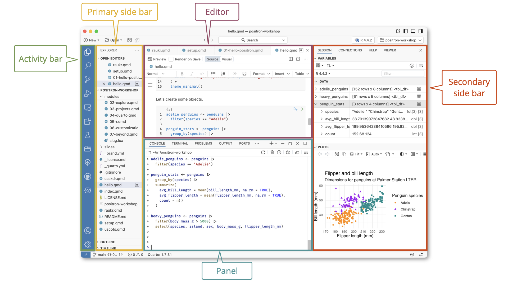
See the Positron documentation for more information on the layout.

YAML

The top portion of your Quarto file (between the three dashed lines) is called YAML. It stands for “YAML Ain’t Markup Language”. It is a human friendly data serialization standard for all programming languages. All you need to know is that this area is called the YAML (we will refer to it as such) and that it contains meta information about your document.

Important

Open the Quarto (.qmd) file in your workspace, change the author name to your name, and render the document. Examine the rendered document.

Loading {renv} cached packages

Reproducible environments

Project-oriented workflows benefit from reproducible environments. There are three major benefits to reproducible environments:

Isolation: Each project has its own set of packages, avoiding conflicts between projects.
Portability: Projects can be shared with others without worrying about package versions or dependencies.
Reproducibility: Projects can be run on different systems with the same results, as all package versions are controlled.

In this class, we use the {renv} package to manage reproducible environments. It allows us to create isolated project environments with specific package versions, ensuring that everyone in the class can reproduce the same results, whether you are using Posit Workbench or your own computer.

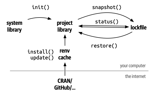
A workflow diagram showing how renv works in a project-oriented workflow — {renv} workflow. Source: {renv} documentation

While the overall workflow is somewhat complex, we keep things simple in this class. We pre-configure each assignment repo’s lockfile to list the minimum required packages that need to be installed. To access these packages, when you first clone the repo run

renv::restore()

This will retrieve installed packages from your cache folder, or download and install packages you have not used before.

Committing changes

Now, go to the Git pane in your Positron instance. This will be in the sidebar through the Git icon.

If you have made changes to your Quarto (.qmd) file, you should see it listed here. Click on it to view the difference between the last committed state of the document and its current state including changes. You should see deletions in red and additions in green.

If you’re happy with these changes, we’ll prepare the changes to be pushed to your remote repository. First, stage your changes by selecting each file to be included in the commit (the + icon). Next, write a meaningful commit message (for instance, “updated author name”) in the Commit message box. Finally, click Commit. Note that every commit needs to have a commit message associated with it.

You don’t have to commit after every change, as this would get quite tedious. You should commit states that are meaningful to you for inspection, comparison, or restoration.

In the first few assignments we will tell you exactly when to commit and in some cases, what commit message to use. As the semester progresses we will let you make these decisions.

Push changes

Now that you have made an update and committed this change, it’s time to push these changes to your repo on GitHub.

In order to push your changes to GitHub, you must have staged your commit to be pushed. Click on Push.

Packages

In this homework we will work with two packages:

{tidyverse} which is a collection of packages for doing data analysis in a “tidy” way, and
{scales} which provides tools for formatting the labels on a plot.

Render the document which loads these two packages with the library() function.

Note

The rendered document will include a message about which packages the {tidyverse} package is loading along with it. It’s just R being informative, a message does not indicate anything is wrong (it’s not a warning or an error).

{tidyverse} is a meta-package. When you load it you get nine packages loaded for you:

{ggplot2}: for data visualization
{dplyr}: for data wrangling
{tidyr}: for data tidying and rectangling
{readr}: for reading and writing data
{tibble}: for modern, tidy data frames
{stringr}: for string manipulation
{forcats}: for dealing with factors
{lubridate}: for dealing with dates/times
{purrr}: for iteration with functional programming

The message that’s printed when you load the package tells you which versions of these packages are loaded as well as any conflicts they may have introduced, e.g., the filter() function from {dplyr} has now masked (overwritten) the filter() function available in base R (and that’s ok, we’ll use dplyr::filter() anyway).

You can now Render your template document and see the results.

Data

The World Bank maintains an extensive database of global development data. The data frame we will be working with today contains a handful of those development indicators, measured for every country over a span of years.

The data are stored as a CSV (Comma-Separated Values) file in the data folder of your repository.

Let’s also load the packages in the Console. You can do this by either typing the following in the console or clicking on the Run cell (triangle) on the code cell that loads the packages.

library(tidyverse)
library(scales)

Next we import the data and save it as an object called wdi.

wdi <- read_csv("data/wdi.csv")

The data contains the following variables:

country - name of the country
iso2c and iso3c - standardized two and three-letter designations respectively for each country
region - the World Bank classifies countries into seven distinct geographic regions
year - the year for which the measures are reported
life_exp - life expectancy at birth, measured in total (years)
pop - total population
gdp - GDP per capita (inflation-adjusted 2015 U.S. dollars)

If you want to know more about a function or a dataset that comes from a package, type a question mark before its name in your console.

?read_csv

A question mark before the name of an object will always bring up its help file. This command must be run in the console. Alternatively, you can use the help() function.

help(read_csv)

Exercises

Exercise 1

Use the glimpse() function to get an overview (or “glimpse”) of the data. How many rows and how many columns does wdi have? What does each row represent? Add your responses to your report.

When you’re done, commit your changes with the commit message “Added answer for Ex 1”,

Then, push these changes.

Data visualization with {ggplot2}

{ggplot2} is the package and ggplot() is the core function used to create a plot. It is loaded as part of the tidyverse, so you do not need to load it separately.

Plots are built up in layers:

ggplot() creates the initial base coordinate system, and we add layers to that base. We first specify the data set we will use with data = wdi.
The mapping argument defines which variables in the data frame are mapped with specific aesthetics, or the visual channels used to communicate information in the graph, e.g. the x axis will represent the variable gdp and the y axis will represent the variable life_exp.
The geom_*() function specifies the type of plot we want to use to represent the data. geom_point() creates a plot where each observation is represented by a point.

Note that layers are joined together with a +, not a pipe.

Exercise 2

Create a scatterplot of life_exp (on the \(y\) axis) versus gdp (on the \(x\) axis). Add an informative title and labels for the \(x\) and \(y\) axes. Then explain the warning message R produces when you render this plot.

Below is the code you will need to get started. Basically, most of the answer is already given, but you need to include the relevant bits in your document, fill in the labels, successfully render it, and view the results.

ggplot(
  data = wdi,
  mapping = aes(x = gdp, y = life_exp)
) +
  geom_point() +
  labs(
    x = "___",
    y = "___",
    title = "___"
  )

Warning: Removed 639 rows containing missing values or values outside the scale range
(`geom_point()`).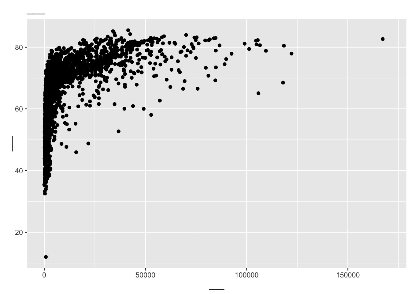

In the narrative below your code chunk, explain in one or two sentences what the warning means.

Tip

The warning refers to rows that could not be drawn. What would make a row impossible to place on this plot?

This is a good place to pause, render, and commit changes with the commit message “Added answer for Ex 2.”

Then, push these changes when you’re done.

Exercise 3

An aesthetic is a visual property of one of the objects in your plot. Commonly used aesthetic options are:

color
fill
shape
size
alpha (transparency)

Recreate your plot from Exercise 2, but this time also map the color of the points to the variable region. Update your title so it reflects the new aesthetic. Then, in one or two sentences, describe what the colors reveal that the previous plot did not.

This is another good place to pause, render, and commit changes with the commit message “Added answer for Ex 3.”

Then, push these changes when you’re done.

Exercise 4

Expand on your plot from Exercise 3 by mapping the size of the points to pop and setting the transparency of the points to alpha = 0.5.

Setting vs. mapping

size = pop maps an aesthetic to a variable, so it goes inside aes(). alpha = 0.5 sets an aesthetic to a fixed value, so it goes inside geom_point() but outside of aes().

You should pause again, render, commit changes with the commit message “Added answer for Ex 4”.

Then, push.

Exercise 5

The plot is getting crowded. Expand on your plot from Exercise 4 by using facet_wrap() to draw the association between GDP and life expectancy separately for each region. Then make the plot easier to read by:

Transforming the \(x\) axis to use log-10 scaling (this accounts for the skewness in the GDP variable)
Formatting the \(x\) axis and size guide labels so they are legible
Removing the legend for region, since it duplicates the facet labels
Moving the remaining legend to the top of the plot and giving it a clear title

Tip

facet_wrap() takes a set of variables, e.g. facets = vars(region).
For the axes, you can transform the scales using scale_x_log10() and scale_size_area(). The labels can be modified using the {scales} package, specifically the label_currency(), label_number(), and cut_short_scale() functions.
To drop a legend, use guide = "none" in the relevant scale_*() function. To move a legend, use theme(legend.position = ...).

In the narrative below the code chunk, briefly comment on what you notice about the association between GDP and life expectancy across regions (one or two sentences is fine!).

You should pause again, render, commit changes with the commit message “Added answer for Ex 5”.

Then, push.

Exercise 6

Scatterplots are not the only geometry available to us.

Create side-by-side box plots of life_exp by region. Many of the region labels will overlap and be difficult to read, so orient the box plots horizontally. Label your axes and give the plot an informative title.

In the narrative below the code chunk, comment on what this graph tells you about life expectancy around the world (one or two sentences is fine!).

Render, commit changes with the commit message “Added answer for Ex 6”.

Then, push.

You’re done with the data analysis exercises, but we’d like to do one more thing to customize the look of the report.

Resize your figures

We can customize the output from a particular R cell by including options in the header that will override any global settings.

Exercise 7

In the R chunks you wrote for Exercises 2-6, customize the settings by modifying the options** in the R chunks used to create those figures.**

For Exercises 2, 3, and 4, we want wide figures. We can use fig-height and fig-width in the options to adjust the height and width of figures. Modify the chunks in Exercises 2-4 to be as follows:

```{r}
#| label: ex2-cell-label
#| fig-height: 4
#| fig-width: 7

# Your code that created the figure
```

Note

Code cell labels need to be unique or you will get an error when you render the document. Make sure to fix the label in each cell to be unique to the specific exercise. Even better, choose something substantive yet simple that describes the cell rather than ex2-cell-label.

For Exercise 5, modify your figure to have fig-height of 6 and fig-width of 8. For Exercise 6, modify your figure to have fig-height of 4 and fig-width of 7.

Now, save and render.

Once you’ve created this PDF file, you’re done!

Commit all remaining changes with the commit message “Done with Homework 0!”.

Then push.

Submission

Once you are finished with the homework, you will submit your final PDF document to Gradescope.

Warning

Before you wrap up the assignment, make sure all documents are updated on your GitHub repo. We will be checking these to make sure you have been practicing how to commit and push changes.

You must turn in a PDF file to the Gradescope page by the submission deadline to be considered “on time”.

To submit your assignment:

Go to http://www.gradescope.com and click Log in in the top right corner.
Click School Credentials \(\rightarrow\) Cornell University NetID and log in using your NetID credentials.
Click on your INFO 5001 course.
Click on the assignment, and you’ll be prompted to submit it.
Mark all the pages associated with exercise. All the pages of your homework should be associated with at least one question (i.e., should be “checked”).

Note

Select all pages of your .pdf submission to be associated with Exercise 7.
Select all pages of your .pdf submission to be associated with the “Workflow & formatting” question.

Grading (50 pts)

This assignment does not count towards your final grade

This assignment is designed to familiarize you with the course infrastructure and workflow. We will collect it and grade it as if it was the real thing, but it will not count towards your final grade.

Component	Points
Ex 1	5
Ex 2	8
Ex 3	5
Ex 4	5
Ex 5	9
Ex 6	5
Ex 7	5
Workflow & formatting	8

Note

The “Workflow & formatting” component assesses the reproducible workflow. This includes:

Having at least 3 informative commit messages
Following {tidyverse} code style
All code being visible in rendered PDF without automatic wrapping (no more than 80 characters)
Appropriate figure sizing, and figures with informative labels and legends

Acknowledgments

The workflow portions of this assignment are derived from Data Science in a Box and licensed under CC BY-SA 4.0.
The data visualization exercises are inspired by Bechdel + data visualization.