AE 07: Using {duckdb} for Lego® data
Suggested answers
Packages
We will use the following packages in this application exercise.
- {tidyverse}: For data import, wrangling, and visualization.
- {duckdb}: To query a DuckDB.
- {dbplyr}: To translate our {dplyr} and {tidyr} functions to SQL.
- {scales}: Formatting graph labels.
Lego®
The Lego® Group was founded in 1932 by Ole Kirk Kristiansen. “LEGO” is an abbreviation of the two Danish words “leg” and “godt”, meaning “play well”. In the 1950s, the Lego® Group launched its most popular line of toys: LEGO Bricks. The company has produced over 600 billion LEGO bricks since its founding, and has become one of the most popular toys in the world. As of 2026, the company has produced over 26,000 different sets and over 60,000 unique parts. Hobbyists and afficianados of the toy have created a vibrant community around collecting and building with LEGO bricks, and there are many online resources for sharing and discussing LEGO-related content.
One of the most popular resources for LEGO fans is Rebrickable, a website that provides a comprehensive database of LEGO sets, parts, and themes. The website allows users to search for specific sets or parts, create and share their own collections, and connect with other LEGO enthusiasts. Rebrickable also provides a variety of tools and resources for building and customizing LEGO creations, making it a valuable resource for both casual fans and serious collectors. They publish a comprehensive dataset of LEGO-related data, which can be accessed through their website or downloaded in bulk. Unfortunately the dataset is difficult to work with in its raw form, as it is provided as a collection of CSV files that are not optimized for analysis. In total there are over 1.7 million rows of data split across 12 tables.
To solve these issues, we will utilize a DuckDB that contains all the tables provided by Rebrickable. This dataset can be access from data/lego.duckdb.
Connect to the database
Demonstration: Connect to the local database and identify the tables.
con <- duckdb(dbdir = "data/lego.duckdb") |>
  dbConnect()

dbListTables(con)
[1] "colors" "elements" "inventories"
[4] "inventory_minifigs" "inventory_parts" "inventory_sets"
[7] "minifigs" "part_categories" "part_relationships"
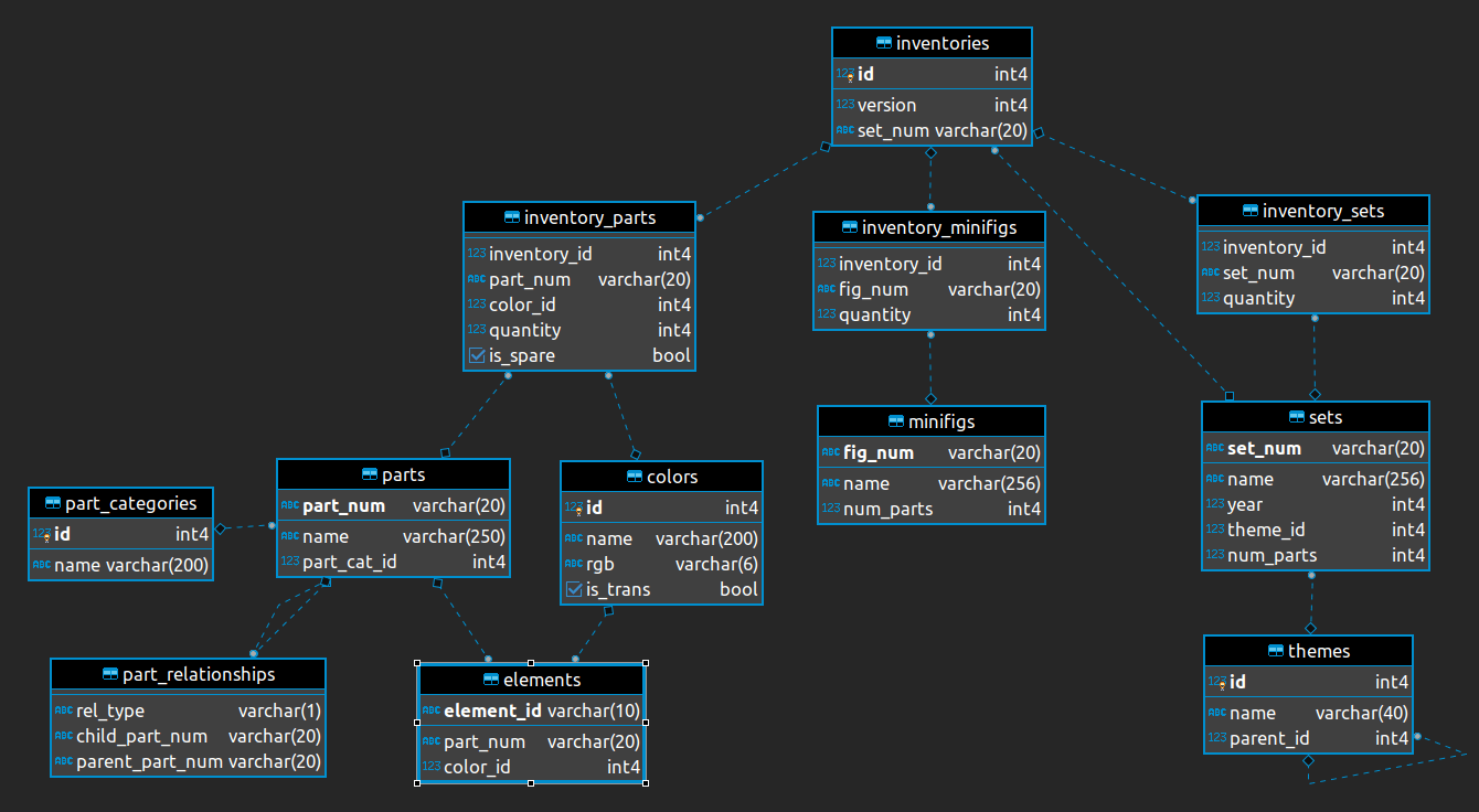
[10] "parts" "sets" "themes" The database has the following relational structure:
Demonstration: Use tbl() to create an object that represents each database table. This will allow us to use {dbplyr} to translate our code to the corresponding SQL query.
lego_colors <- tbl(con, "colors")
lego_elements <- tbl(con, "elements")
lego_inventories <- tbl(con, "inventories")
lego_inventory_minifigs <- tbl(con, "inventory_minifigs")
lego_inventory_parts <- tbl(con, "inventory_parts")
lego_inventory_sets <- tbl(con, "inventory_sets")
lego_minifigs <- tbl(con, "minifigs")
lego_part_categories <- tbl(con, "part_categories")
lego_part_relationships <- tbl(con, "part_relationships")
lego_parts <- tbl(con, "parts")
lego_sets <- tbl(con, "sets")
lego_themes <- tbl(con, "themes")
Examine the relational structure of the database
Your turn: Identify the primary key for colors. What is its foreign key in the elements and inventory_parts tables?
Add response here. The primary key for colors is id. The foreign key in both the elements and inventory_parts tables that corresponds to this primary key is color_id.
Your turn: Identify the primary key for themes. What does the dashed line between themes and themes mean?
Add response here.
lego_themes# A query: ?? x 3
# Database: DuckDB 1.5.5 [root@Darwin 27.0.0:R 4.6.1//Users/bcs88/Projects/info-5001/course-site/ae/data/lego.duckdb]
id name parent_id
<dbl> <chr> <dbl>
1 1 Technic NA
2 3 Competition 1
3 4 Expert Builder 1
4 16 RoboRiders 1
5 17 Speed Slammers 1
6 18 Star Wars 1
7 19 Supplemental 1
8 20 Throwbot Slizer 1
9 21 Universal Building Set 1
10 22 Creator NA
# ℹ more rowsThe primary key for themes is id. The dashed line between themes and themes indicates that there is a self-referential relationship between the two tables. Specifically, the parent_id column in the themes table is a foreign key that references the id column in the same table, allowing for hierarchical relationships between themes.
Translate some basic SQL queries
Your turn: Explain what each of the following SQL queries does, and recreate them using {dbplyr}.
SELECT "sets".*
FROM "sets"
WHERE (num_parts > 200.0)
Add response here. Filter the sets table to only keep rows where the number of parts in the set is greater than 200.
lego_sets |>
  filter(num_parts > 200) |>
  show_query()
<SQL>
SELECT *
FROM "sets"
WHERE (num_parts > 200.0)SELECT "year", AVG(num_parts) AS num_parts
FROM "sets"
GROUP BY "year"Add response here. Summarize the sets table by year, calculating the average number of parts in sets for each year.
lego_sets |>
group_by(year) |>
summarize(num_parts = mean(num_parts, na.rm = TRUE)) |>
show_query()<SQL>
SELECT "year", AVG(num_parts) AS num_parts
FROM "sets"
GROUP BY "year"lego_sets |>
group_by(year) |>
summarize(num_parts = mean(num_parts)) |>
show_query()Warning: Missing values are always removed in SQL aggregation functions.
Use `na.rm = TRUE` to silence this warning
This warning is displayed once every 8 hours.<SQL>
SELECT "year", AVG(num_parts) AS num_parts
FROM "sets"
GROUP BY "year"Change over time in set complexity
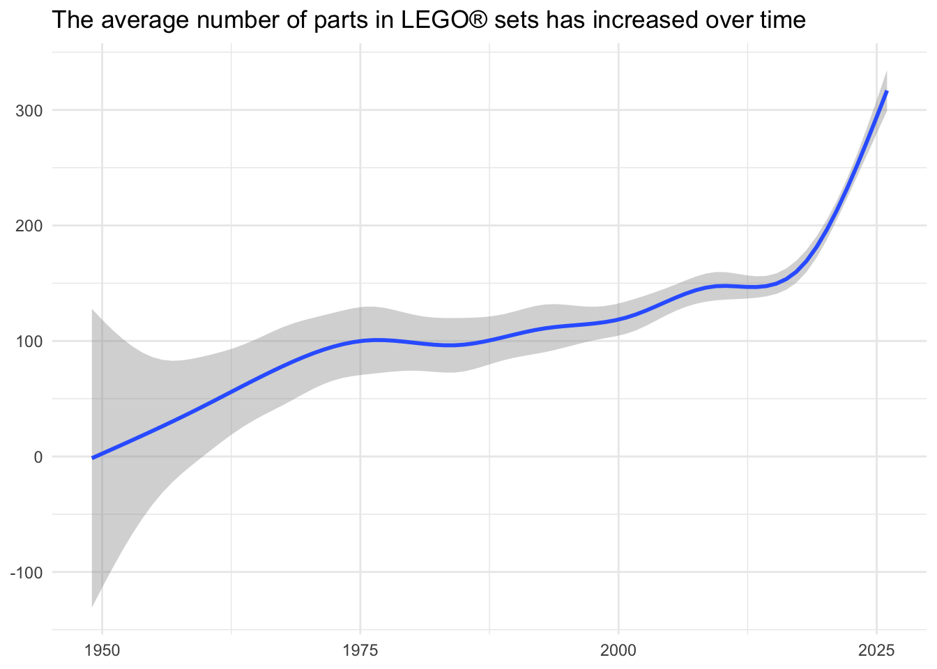
Now let’s examine how the complexity of LEGO® sets has changed over time. We can use the number of parts in a set as a proxy for its complexity.
Demonstration: Visualize the change over time in the number of parts in sets.
lego_sets |>
  ggplot(mapping = aes(x = year, y = num_parts)) +
  geom_smooth() +
  labs(
    title = "The average number of parts in LEGO® sets has increased over time",
    x = NULL,
    y = NULL
  )
Visualize the average set size over time
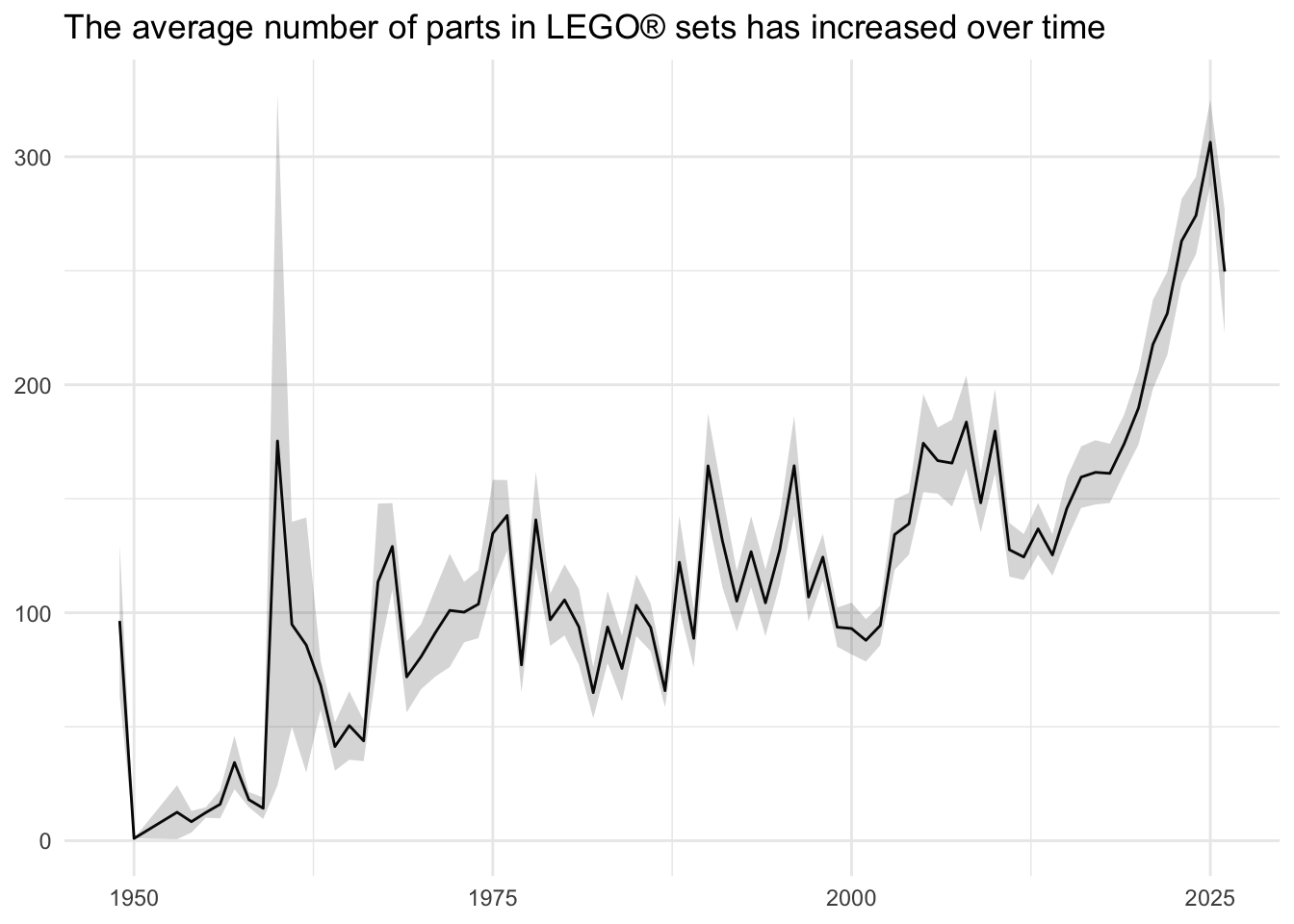
Your turn: Visualize the change over time in the average number of parts in sets. For each year, calculate the average number of parts in sets released that year, and visualize the change in this value over time.
lego_sets |>
  summarize(
    num_parts_mean = mean(num_parts, na.rm = TRUE),
    se = sd(num_parts, na.rm = TRUE) / sqrt(n()),
    .by = year
  ) |>
  ggplot(mapping = aes(x = year, y = num_parts_mean)) +
  geom_line() +
  geom_ribbon(
    mapping = aes(ymin = num_parts_mean - se, ymax = num_parts_mean + se),
    alpha = 0.2
  ) +
  labs(
    title = "The average number of parts in LEGO® sets has increased over time",
    x = NULL,
    y = NULL
  )
Calculate a rolling average
The line graph is a bit noisy due to annual fluctuations in the average number of parts in sets. One method to smooth this out is to create a rolling average. This generates a sliding window across the timespan, averaging the values for each observation within that span as it moves across the time period.
There are several ways to accomplish this task in R. One popular implementation in the {zoo} package provides drop in functions for calculating rolling means, maximums, medians, and sums. Unfortunately these functions have not been translated by {dbplyr} for use with SQL databases.
Fortunately SQL has direct support for these operations through so-called window functions. In order to utilize them, we need to identify the boundaries of the frame (the sliding window). We can do that using window_frame().
Demonstration: Calculate a rolling five-year average set size.
roll_lego <- lego_sets |>
  summarize(
    num_parts_mean = mean(num_parts, na.rm = TRUE),
    .by = year
  ) |>
  window_frame(-2, 2) |>
  mutate(roll_mean = mean(num_parts_mean, na.rm = TRUE))

show_query(roll_lego)
Warning: Windowed expression `AVG(num_parts_mean)` does not have explicit order.
ℹ Please use `arrange()`, `window_order()`, or `.order` to make deterministic.<SQL>
SELECT
*,
AVG(num_parts_mean) OVER (ROWS BETWEEN 2 PRECEDING AND 2 FOLLOWING) AS roll_mean
FROM (
SELECT "year", AVG(num_parts) AS num_parts_mean
FROM "sets"
GROUP BY "year"
) AS q01collect(roll_lego)Warning: Windowed expression `AVG(num_parts_mean)` does not have explicit order.
ℹ Please use `arrange()`, `window_order()`, or `.order` to make deterministic.# A tibble: 76 × 3
year num_parts_mean roll_mean
<dbl> <dbl> <dbl>
1 2008 184. 139.
2 2015 146. 139.
3 2001 87.9 130.
4 2004 139. 118.
5 1986 93.6 122.
6 2014 125. 108.
7 1996 164. 80.5
8 1958 18.0 82.9
9 1950 1 87.5
10 1980 106. 80.1
# ℹ 66 more rowsWarning: Windowed expression `AVG(num_parts_mean)` does not have explicit order.
ℹ Please use `arrange()`, `window_order()`, or `.order` to make deterministic.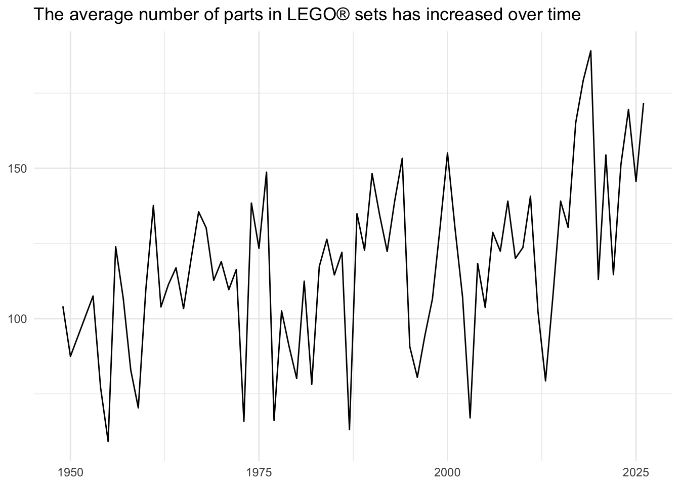
Unfortunately this is only partially correct. Recall that SQL tables have no intrinsic row-order. Every time you run a query, the rows you obtain can be in a different order every time. In order to ensure we correctly calculate the five-year window, we need to define the order of the rows for the table. We can do this by either using arrange() to explicitly order the rows before using the window function, or use window_order() to define the order.
roll_lego <- lego_sets |>
  summarize(
    num_parts_mean = mean(num_parts, na.rm = TRUE),
    .by = year
  ) |>
  window_order(year) |>
  window_frame(-2, 2) |>
  mutate(roll_mean = mean(num_parts_mean, na.rm = TRUE))

show_query(roll_lego)
<SQL>
SELECT
*,
AVG(num_parts_mean) OVER (ORDER BY "year" ROWS BETWEEN 2 PRECEDING AND 2 FOLLOWING) AS roll_mean
FROM (
SELECT "year", AVG(num_parts) AS num_parts_mean
FROM "sets"
GROUP BY "year"
) AS q01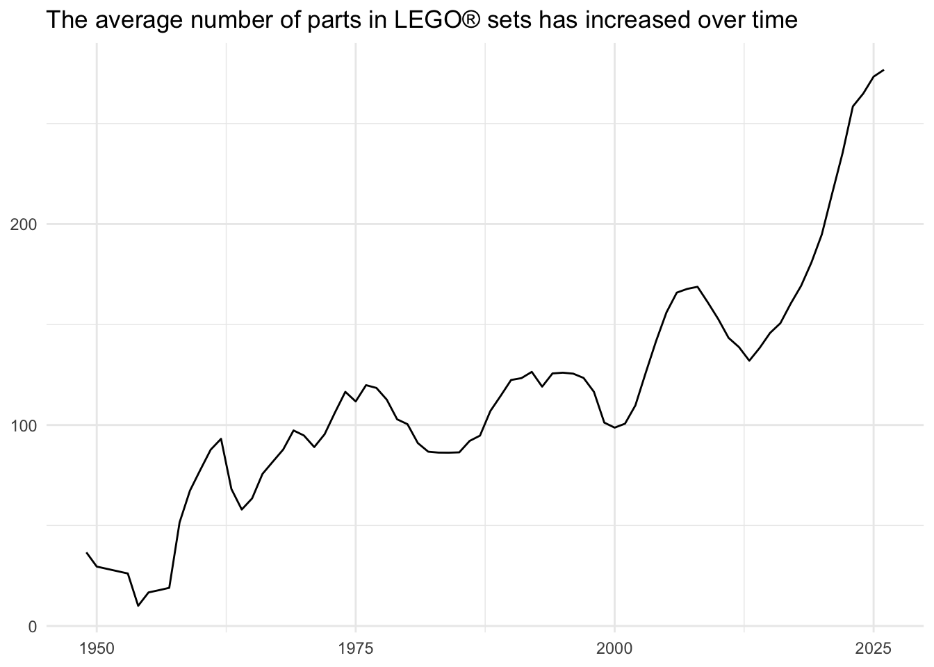
Use case for SQL: Data-driven dashboards
Even when you are not writing SQL queries by hand, or converting from R code, SQL has a number of useful applications. {querychat} is a package for R or Python that enables natural language exploration of tabular data, using SQL and large language models (LLMs) to generate queries and visualizations. This allows users to ask questions about their data in natural language, and receive answers in the form of SQL queries and visualizations.
Demonstration: Use the Lego Explorer app to explore the Lego® dataset.
- What is the parent theme with the most “children” themes?
- Change over time in set complexity
sessioninfo::session_info()─ Session info ───────────────────────────────────────────────────────────────
setting value
version R version 4.6.1 (2026-06-24)
os macOS Golden Gate 27.0
system aarch64, darwin23
ui X11
language (EN)
collate en_US.UTF-8
ctype en_US.UTF-8
tz America/New_York
date 2026-09-25
pandoc 3.10 @ /Applications/Positron.app/Contents/Resources/app/quarto/bin/tools/aarch64/ (via rmarkdown)
quarto 1.10.18 @ /Applications/quarto/bin/quarto
─ Packages ───────────────────────────────────────────────────────────────────
! package * version date (UTC) lib source
P blob 1.3.0 2026-01-14 [?] RSPM
P cli 3.6.6 2026-04-09 [?] RSPM
P DBI * 1.3.0 2026-02-25 [?] RSPM
P dbplyr * 2.6.0 2026-06-17 [?] RSPM
P digest 0.6.39 2025-11-19 [?] RSPM
P dplyr * 1.2.1 2026-04-03 [?] RSPM
P duckdb * 1.5.5 2026-07-25 [?] RSPM
P evaluate 1.0.5 2025-08-27 [?] RSPM
P farver 2.1.2 2024-05-13 [?] RSPM
P fastmap 1.2.0 2024-05-15 [?] RSPM
P forcats * 1.0.1 2025-09-25 [?] RSPM
P generics 0.1.4 2025-05-09 [?] RSPM
P ggplot2 * 4.0.3 2026-04-22 [?] RSPM
P glue 1.8.1 2026-04-17 [?] RSPM
P gtable 0.3.6 2024-10-25 [?] RSPM
P here 1.0.2 2025-09-15 [?] RSPM
P hms 1.1.4 2025-10-17 [?] RSPM
P htmltools 0.5.9 2025-12-04 [?] RSPM
P htmlwidgets 1.6.4 2023-12-06 [?] RSPM
P jsonlite 2.0.0 2025-03-27 [?] RSPM
P knitr 1.51 2025-12-20 [?] RSPM
P labeling 0.4.3 2023-08-29 [?] RSPM
P lattice 0.22-9 2026-02-09 [?] CRAN (R 4.6.1)
P lifecycle 1.0.5 2026-01-08 [?] RSPM
P lubridate * 1.9.5 2026-02-04 [?] RSPM
P magrittr 2.0.5 2026-04-04 [?] RSPM
P Matrix 1.7-5 2026-03-21 [?] CRAN (R 4.6.1)
P mgcv 1.9-4 2025-11-07 [?] CRAN (R 4.6.1)
P nlme 3.1-169 2026-03-27 [?] CRAN (R 4.6.1)
P otel 0.2.0 2025-08-29 [?] RSPM
P pillar 1.11.1 2025-09-17 [?] RSPM
P pkgconfig 2.0.3 2019-09-22 [?] RSPM
P purrr * 1.2.2 2026-04-10 [?] RSPM
P R6 2.6.1 2025-02-15 [?] RSPM
P RColorBrewer 1.1-3 2022-04-03 [?] RSPM
P readr * 2.2.0 2026-02-19 [?] RSPM
renv 1.2.2 2026-04-16 [1] RSPM (R 4.6.1)
P rlang 1.3.0 2026-07-05 [?] RSPM
P rmarkdown 2.31 2026-03-26 [?] RSPM
P rprojroot 2.1.1 2025-08-26 [?] RSPM
P S7 0.2.2 2026-04-22 [?] RSPM
P scales * 1.4.0 2025-04-24 [?] RSPM
P sessioninfo 1.2.4 2026-06-04 [?] RSPM
P stringi 1.8.9 2026-08-04 [?] RSPM
P stringr * 1.6.0 2025-11-04 [?] RSPM
P tibble * 3.3.1 2026-01-11 [?] RSPM
P tidyr * 1.3.2 2025-12-19 [?] RSPM
P tidyselect 1.2.1 2024-03-11 [?] RSPM
P tidyverse * 2.0.0 2023-02-22 [?] RSPM
P timechange 0.4.0 2026-01-29 [?] RSPM
P tzdb 0.5.0 2025-03-15 [?] RSPM
P utf8 1.2.6 2025-06-08 [?] RSPM
P vctrs 0.7.3 2026-04-11 [?] RSPM
P withr 3.0.3 2026-06-19 [?] RSPM
P xfun 0.60 2026-07-09 [?] RSPM
P yaml 2.3.12 2025-12-10 [?] RSPM
[1] /Users/bcs88/Projects/info-5001/course-site/renv/library/macos/R-4.6/aarch64-apple-darwin23
[2] /Users/bcs88/Library/Caches/org.R-project.R/R/renv/sandbox/macos/R-4.6/aarch64-apple-darwin23/46003b10
* ── Packages attached to the search path.
P ── Loaded and on-disk path mismatch.
──────────────────────────────────────────────────────────────────────────────