Quiz 03
Quiz
Overview
Quiz 3 will be held on December 1st in-class. It will be a 75 minute in-person, timed quiz.
The quiz will cover all material through the end of week 13 (interactive web applications with Shiny), with an explicit emphasis on content taught since week 9 (reproducible reporting with Quarto). It will consist of a series of short answer and free response questions. Questions are designed to evaluate your understanding of concepts and methods. You may be asked to answer conceptual questions, interpret visualizations, interpret code and output, and/or write code by hand.
Students with SDS accommodations
Students who have registered SDS accommodations related to timed assignments are implemented by the SDS Alternative Testing Program. You will receive separate instructions from SDS about how to take the quiz with your accommodations. If you have any questions about your accommodations, please contact SDS directly.
Students with religious or other accommodations
If you require an accommodation for quiz 03 on the basis of religious observances, athletics, military service, or another accommodation listed on the course syllabus, please contact us at soltoffbc@cornell.edu by November 20. Any accommodation requests received after this date are unlikely to be approved.
Rules & Notes
Academic Integrity
- A student shall in no way misrepresent his or her work.
- A student shall in no way fraudulently or unfairly advance his or her academic position.
- A student shall refuse to be a party to another student’s failure to maintain academic integrity.
- A student shall not in any other manner violate the principle of academic integrity.
- This is an individual assignment. Everything in the quiz is for your eyes only.
- The quiz will be held in-person. All responses will be written by hand and submitted on paper.
- You may not use any electronic devices during the quiz.1 This includes laptops, tablets, phones, smartwatches, etc.
- You may not use any physical materials during the quiz. This includes textbooks, notes, calculators, etc. Any required information will be provided in the quiz.
Submission
- All responses will be submitted on paper using the provided forms. Quizzes will be evaluated and returned to you via Gradescope.
Grading
Each quiz is weighted equally. There will be three quizzes in total, so each quiz is worth 10% of your final grade.
Practice problems
NoteInstructions
Below are some practice problems you may complete in order to prepare for the quiz. The suggested solution is hidden below each exercise. Try to solve the problem on your own before looking at the solution.
-
For each scenario, would you write an R script (
.R) or a Quarto document (.qmd)? Briefly justify each choice.- A set of helper functions that clean Tidy Tuesday data files, which several of your analyses will load with
source(). - A weekly report for the Cornell Dining management team summarizing coffee sales, with charts and written interpretation.
- A data pipeline step that downloads the latest data, cleans it, and writes a
.csvfile to disk every night. - A homework assignment in which you must explain your reasoning next to the code that supports it.
NoteSuggested solution-
.Rscript. Shared functions belong in a script that other files cansource(); there is no narrative to render. -
.qmd. The audience needs prose, figures, and tables combined into a rendered report, and re-rendering each week keeps it reproducible. -
.Rscript. A pipeline step runs programmatically (e.g.Rscriptorsource()) and produces a file, not a document. -
.qmd. Code, output, and explanation need to sit together in one rendered document.
Other answers can be reasonable with a sound justification. The real answer is often “it depends.”
- A set of helper functions that clean Tidy Tuesday data files, which several of your analyses will load with
-
Fill in the blanks to specify a logistic regression model, estimated with base R’s
glm()function, that predicts a binary outcome.lr_spec <- ________(A)________ |> set_engine(________(B)________) |> set_mode(________(C)________)Then explain the purpose of
set_engine(). Why does {parsnip} separate the model type from the engine?NoteSuggested solution-
(A)
logistic_reg() -
(B)
"glm" -
(C)
"classification"
set_engine()specifies the computational engine (the package or function) that actually fits the model. The same model type can be estimated by several engines (logistic_reg()can use"glm","glmnet","stan","keras", …), each with its own syntax. Separating the model type from the engine gives you one consistent interface, so you can swap engines without rewriting the rest of your code. -
(A)
-
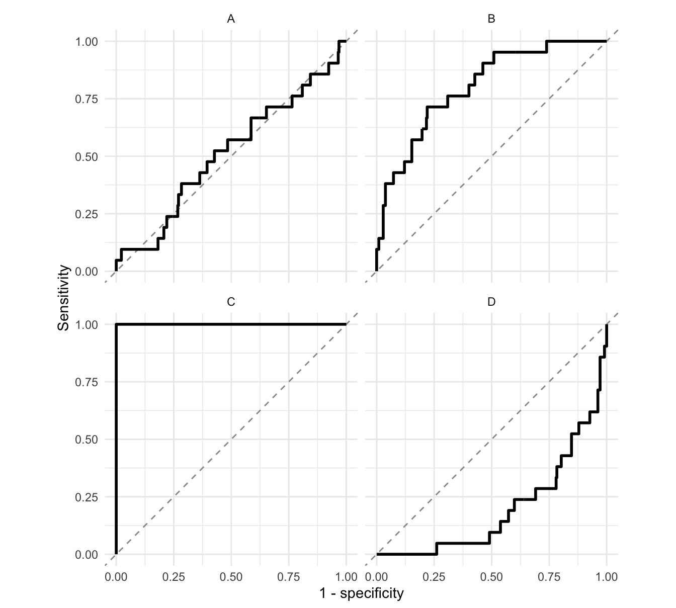
Each panel below shows the ROC curve for a different classifier predicting whether a coffee in the Coffee Quality Institute ratings is top rated (a total cupping score of 85 or higher), evaluated on the same test set. Match each panel to its approximate ROC AUC: 0.2, 0.5, 0.8, or 1.0. Use each value once.
NoteSuggested solution- A: 0.5. The curve hugs the diagonal; the classifier is no better than random guessing (it literally is random guessing).
- B: 0.8. The curve bows toward the upper-left corner but not all the way. This is a logistic regression fit to the training data.
- C: 1.0. The curve goes straight up to sensitivity = 1 before moving right: a perfect classifier.
- D: 0.2. The curve sits below the diagonal; the classifier is worse than guessing (here, the logistic regression’s probabilities reversed).
Actual values: A = 0.51, B = 0.80, C = 1.00, D = 0.20.
-
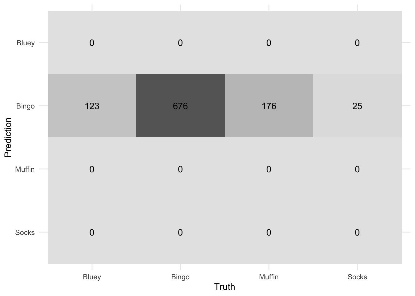
Gallup surveyed 1,000 youths2 asking them which Heeler cousin from hit TV show Bluey is their favourite: Bluey, Bingo, Muffin, or Socks.
This is the confusion matrix for the assessment set using a model predicting individual preferences for Bluey, Bingo, Muffin, or Socks based on other demographic features collected in the survey. Explain what has happened to the model, what might be a contributing factor to these results, and propose a solution to improve the model’s performance.
 NoteSuggested solution
The model predicts Bingo for every respondent. The outcome is heavily imbalanced: Bingo is the favourite of 67.6% of respondents, so always predicting Bingo achieves 67.6% accuracy without learning anything from the predictors.
To address it, rebalance the training data in the recipe, for example
step_downsample()(randomly drop rows from the larger classes until they match the smallest) orstep_upsample()(replicate rows from the smaller classes), both from {themis}. Also evaluate with metrics that are sensitive to the minority classes (e.g. ROC AUC, per-class sensitivity) rather than accuracy alone. -
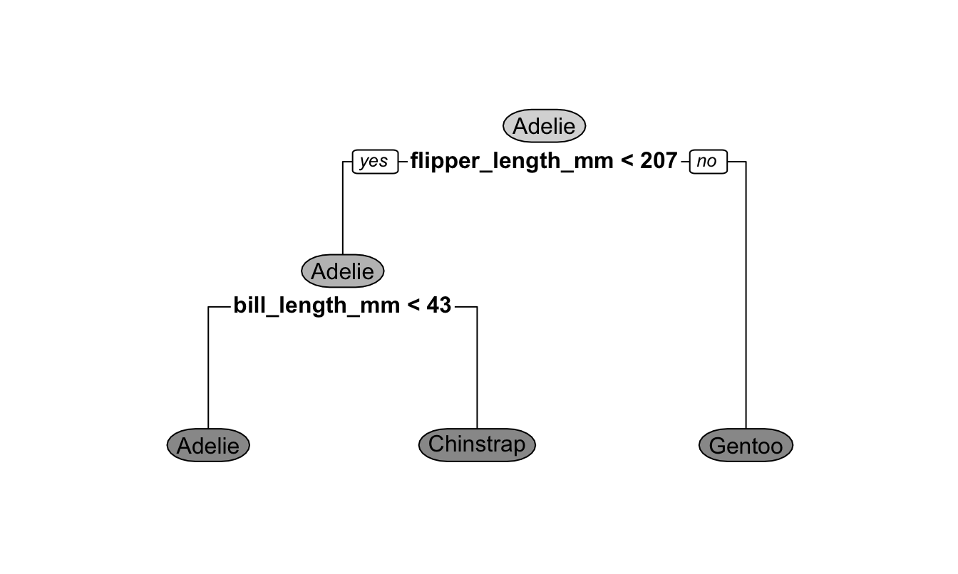
The decision tree below was fit to the Palmer penguins data to predict penguin species from flipper length and bill length (both in millimeters).
-
Predict the species of each penguin:
Penguin Flipper length (mm) Bill length (mm) 1 190 39 2 195 50 How many internal (decision) nodes and how many leaf (terminal) nodes does this tree have? What does each type of node do?
NoteSuggested solutionPenguin 1: flipper length < 207, then bill length < 43 → Adelie. Penguin 2: flipper length < 207, then bill length ≥ 43 → Chinstrap.
-
Two internal nodes (the flipper length split at the root and the bill length split) and three leaf nodes (Adelie, Chinstrap, Gentoo).
- An internal node splits the data on a condition for a single predictor (e.g. “Is flipper length < 207?”) and sends each observation down one branch.
- A leaf node returns the prediction: here the most common species among the training observations that end up there.
-
-
Answer the following questions about tree-based models.
- Bagged trees and random forests both average the predictions of many decision trees, each fit to a bootstrap sample of the training data. What is the primary difference between the two, and why does that difference improve performance?
- In class I asserted that “there is an inverse relationship between model accuracy and model interpretability.” Use a single decision tree and a random forest to explain what this means.
NoteSuggested solutionA random forest considers only a random subset of the predictors (
mtry) at each split, while bagging considers every predictor at every split. In bagging, a few strong predictors dominate the top splits of every tree, so the trees look alike and their errors are correlated. Restricting the candidate predictors decorrelates the trees, and averaging less correlated trees reduces variance more.A single decision tree is easy to interpret: you can draw it and follow the splits to see exactly how a prediction was made, but a single tree has high variance and is usually less accurate. A random forest averages hundreds of trees, which typically improves accuracy, but no person can follow hundreds of trees to explain a prediction. More flexible (and usually more accurate) models tend to be harder to interpret.
-
An LLM is given the text “Cornell University is located in Ithaca, New York, a city known for its” and produces the following probabilities for the next token:
Illustrative next-token probabilities Next token Probability gorges 0.46 waterfalls 0.21 college 0.09 cold 0.06 (all other tokens) 0.18 - Describe how a generative pre-trained transformer (GPT) uses distributions like this one to write an entire response.
- You send the same prompt twice and get two different completions. Using the table, explain why.
NoteSuggested solutionA GPT is trained (pre-trained, on a huge body of text) to predict the next token (a word or piece of a word) given all the text so far. To generate a response it predicts a probability distribution over the next token, picks one, appends it to the text, and repeats, one token at a time, until it produces a stop token.
The model samples the next token from the distribution instead of always taking the most likely one. “gorges” is chosen only 46% of the time; 21% of the time it picks “waterfalls”, and so on. Once one token differs, everything generated after it is conditioned on different text, so the completions diverge.
-
A classmate is labeling congressional bills with this code:
chat <- chat(
  "openai/gpt-6-luna",
  system_prompt = "Label this bill."
)

bill <- "A bill to amend title 18, United States Code, to prohibit
fraudulently representing a product to be maple syrup."

chat$chat(bill)
#> This bill appears to concern consumer protection and criminal law. It would
#> make it a federal crime to fraudulently market a product as maple syrup...
They wanted a single category number from 1 to 20. Using the three prompt engineering best practices from class, describe how you would revise their approach.
NoteSuggested solution-
Put the prompt in a Markdown file (e.g.
prompt.md) and load it withinterpolate_file(). A good labeling prompt is long (all 20 categories with definitions), and a separate file is easier to read, edit, and version than an R string. -
Clearly explain what you want in the system prompt: the task (classify a U.S. congressional bill by its primary policy topic), the full list of 20 categories with their numbers and short definitions, how to break ties (choose the primary topic), and the exact output format (“Respond with only the category number”). Better still, combine with structured output (
type_integer()) so the response is guaranteed to be a number. - Provide examples of descriptions with their correct labels, especially tricky ones. For instance, this maple syrup bill amends the criminal code but the human coders labeled it Agriculture.
-
Put the prompt in a Markdown file (e.g.
-
Problems 9 and 10 use the weather forecast accuracy data from Tidy Tuesday, which compares National Weather Service forecasts to observed temperatures in U.S. cities.
library(shiny) library(bslib) library(tidyverse) forecasts <- read_csv("data/weather-forecasts.csv") ui <- page_sidebar( title = "How accurate are weather forecasts?", sidebar = sidebar( selectInput( inputId = "city", label = "Select a city", choices = sort(unique(forecasts$city)) ) ), plotOutput(outputId = "error_plot"), tableOutput(outputId = "error_table") ) server <- function(input, output, session) { output$error_plot <- renderPlot({ forecasts |> filter(city == input$city) |> ggplot(mapping = aes( x = forecast_hours_before, y = forecast_temp - observed_temp )) + geom_boxplot(mapping = aes(group = forecast_hours_before)) }) output$error_tbl <- renderTable({ forecasts |> filter(city == input$city) |> summarize( mean_abs_error = mean( abs(forecast_temp - observed_temp), na.rm = TRUE ), .by = forecast_hours_before ) }) } shinyApp(ui = ui, server = server)- Describe the role of the
uiand theserverin a Shiny app, using this app as an example. - When you run the app, the plot appears but the table never does. Why? How would you fix it?
NoteSuggested solutionThe UI defines what the user sees in the browser: the layout (
page_sidebar()), the inputs they interact with (selectInput()for the city), and placeholders for outputs (plotOutput(),tableOutput()). The server is the R function that does the work: it reads input values (input$city), computes results, and assigns them tooutput$...withrender*()functions so they fill the matching placeholders.The IDs don’t match. The UI has a placeholder
tableOutput("error_table"), but the server assignsoutput$error_tbl. Shiny never connects them, so the table’s placeholder stays empty. Rename one so both use the same ID (e.g.output$error_table).
- Describe the role of the
-
Your classmate changes the app from problem 9 so users can compare several cities: they add
multiple = TRUEtoselectInput(), change bothfilter()calls tofilter(city %in% input$city), and fix the output ID.- Draw the reactive graph for the app: its reactive sources, conductors (if any), and endpoints, with arrows showing dependencies.
- The filtering code is repeated in both
render*()functions. Rewrite theserverfunction to use a reactive expression so the filtering happens once. - When a user clears every city from the input, the app shows errors. What function would you add to your reactive expression, and how does it fix the problem?
NoteSuggested solutionBefore part (b):
input$city→output$error_plotandinput$city→output$error_table. (One source, two endpoints, no conductor.) After the part (b) rewrite, the graph becomesinput$city→forecasts_city()→ both outputs.-
server <- function(input, output, session) {
  forecasts_city <- reactive({
    req(input$city)
    forecasts |>
      filter(city %in% input$city)
  })

  output$error_plot <- renderPlot({
    forecasts_city() |>
      ggplot(mapping = aes(
        x = forecast_hours_before,
        y = forecast_temp - observed_temp
      )) +
      geom_boxplot(mapping = aes(group = forecast_hours_before))
  })

  output$error_table <- renderTable({
    forecasts_city() |>
      summarize(
        mean_abs_error = mean(
          abs(forecast_temp - observed_temp),
          na.rm = TRUE
        ),
        .by = forecast_hours_before
      )
  })
}
The reactive expression is assigned to a name (not
output$), and it’s called with parentheses,forecasts_city(). req(input$city). When no city is selected,input$cityisNULL, which is not “truthy”, soreq()silently stops the reactive expression and everything downstream of it instead of passing empty data to the plot and table.